Implicit Mechanical Solver
Both linear and nonlinear analytical options, including the selection of static or various types of dynamic solution methods, are offered by the Implicit Mechanical Solver in Ansys LS-DYNA.
Within the platform, engineers can use just one model for a variety of studies as the solver technology it is fully integrated with its Explicit Mechanics equivalent, using the same element and material libraries.
Additionally, the level of application can be increased by effortlessly switching between the implicit and explicit modes during the same simulation.
Applications | Implicit Mechanical
Numerous applications for implicit mechanical analysis exist, including but not limited to:
Consumer Goods
- Drop tests (all kinds)
- Vibration computations
- Acoustical analysis
Aerospace
- Fuselage drop test
- Jet engine startup
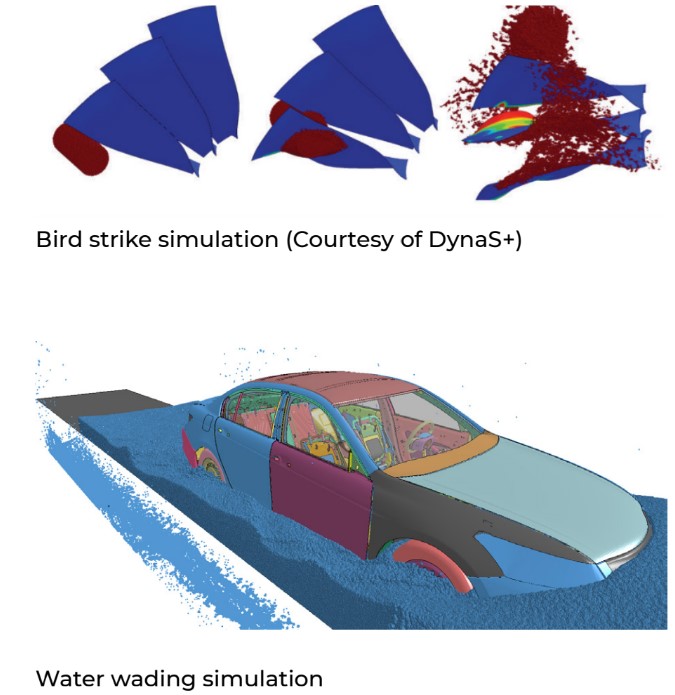
- Bird strike
- Engine vibration
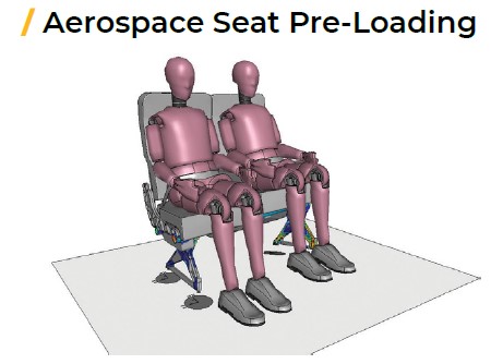
- Analysis of seats
- Satellite stress and vibration tests
Automotive
- Gravity loading
- Dummy seating
- Crash testing
- Hydroplane
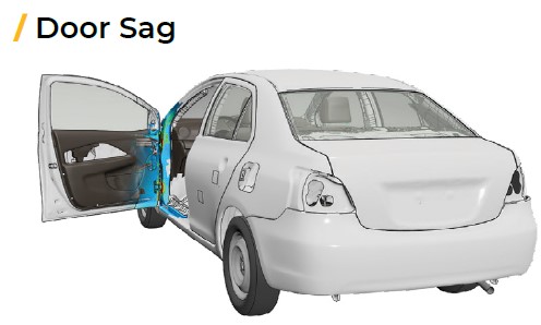
- Door sag
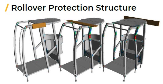
- Roof crush
- Seat pull
Industrial Equipment & Machinery
- Linear and nonlinear analysis
- Buckling, vibration and modal analysis
- Shared memory parallel (SMP)
- Massive parallel processing (MPP)
- Hybrid parallel: combines SMP and MPP
- Scalability that can exceed 10K cores
What distinguishes implicit dynamics from explicit dynamics?
Mass (inertia) and damping have little impact on static analysis. Nodal forces related to mass/inertia and damping are taken into account in dynamic analysis.
In LS-DYNA, a static analysis is performed using an implicit solution. Both the explicit solver and the implicit solver can be used for dynamic analysis.
Each step in a nonlinear implicit analysis must be solved through a number of trial solutions, or iterations, in order to reach equilibrium within a predetermined tolerance. Since the nodal accelerations are immediately solved in explicit analysis, iteration is not necessary.
Explicit analysis time steps must be less than Courant time steps (time it takes a sound wave to travel across an element). There is no inherent limit to implicit transient analysis. Specifically, as it relates to time sequences.
Implicit Mechanics | Time Sequencing
As a result, implicit time steps are typically much bigger than explicit time steps by several orders of magnitude.
In order to perform implicit analysis, a numerical solver must invert the stiffness matrix at least once during each load/time step. It costs a lot to perform this matrix inversion, especially for large models. This step is not required for explicit analyses.
Comparatively speaking to implicit analysis, explicit analysis manages nonlinearities very easily. This would cover how touch and material nonlinearities are handled.
Additionally, engineering applications including hourglass control, bulk viscosity, damping, and element stress. Once the accelerations at time n are known, the velocities at time n+1/2 and the displacements at time n+1 are computed. Displacements lead to strain. Stress results from strain. The process is then repeated.
In explicit dynamic analysis, nodal accelerations are calculated by multiplying the diagonal mass matrix by the net nodal force vector, where the net nodal force incorporates contributions from external sources, directly rather than incrementally (body forces, applied pressure, contact, etc.).