Why Compressible Flow Still Pushes CFD Codes
Whether you’re designing a reusable launch vehicle, a supersonic business jet, or a high-altitude UAV, your simulation probably spans several Mach number regimes in a single model. That variety is what makes compressible flow CFD modeling tricky: solver settings that behave perfectly at Mach 0.2 can stumble once local velocities climb above Mach 1, and vice-versa.
For years, engineers relied on a simple rule: use a pressure-based solver for subsonic conditions and switch to a density-based solver once flow becomes compressible. It worked, but it meant maintaining two workflows, each with its own quirks and validation data. Recent improvements in Ansys Fluent’s numerical methods blur that line.
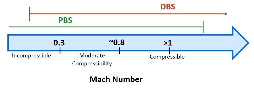
A pressure-based coupled algorithm and better low-Mach pre-conditioning for the density-based simulations enable the use of a single solver for most mixed-Mach problems, yielding accurate solutions while saving considerable time.
From Strict Solver Split to Significant Overlap
| Classic Guidance | What Has Changed | What You Gain |
| Pressure-based solver for Ma ≲ 0.3 | The coupled pressure-based algorithm now handles moderate shocks while maintaining stability | One solver for the entire sub- to transonic flow range |
| Density-based solver for strong shocks | Low-Mach pre-conditioning improves stability down to sub-sonic regime | You can use the density-based solver on mixed-Mach cases without divergence |
In practice, many engineers kick off a fast, pressure-based coupled solve to drive down the residuals and get an initial view of the shock location. Once that baseline solution is saved, they stop the run, switch the case to the density-based solver, re-initialize with the existing flow field, and continue iterating on the same mesh for higher-fidelity shock resolution. Thanks to modern pre-conditioning, the two algorithms overlap in capability, so it is worth trying whichever converges faster for your particular problem.
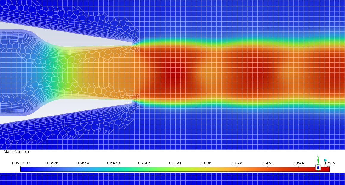
Case Study: Mach 1.3 Jet Exhausting to Ambient Air
Geometry: A converging–diverging axisymmetric nozzle discharges into static air. Engineers meshed the domain with roughly 4 million cells, using about ten cells across the throat. A body-of-influence encloses the expected shock region to better resolve the shock structures.
Solver performance (same mesh):
- Pressure-based SIMPLE – ~600 iterations; converged but shock diamonds were slightly smeared.
- Pressure-based Coupled – ~250 iterations; sharper shocks and realistic momentum decay downstream.
- Density-based Implicit – ~15 000 iterations; best shock definition but highest iteration count.
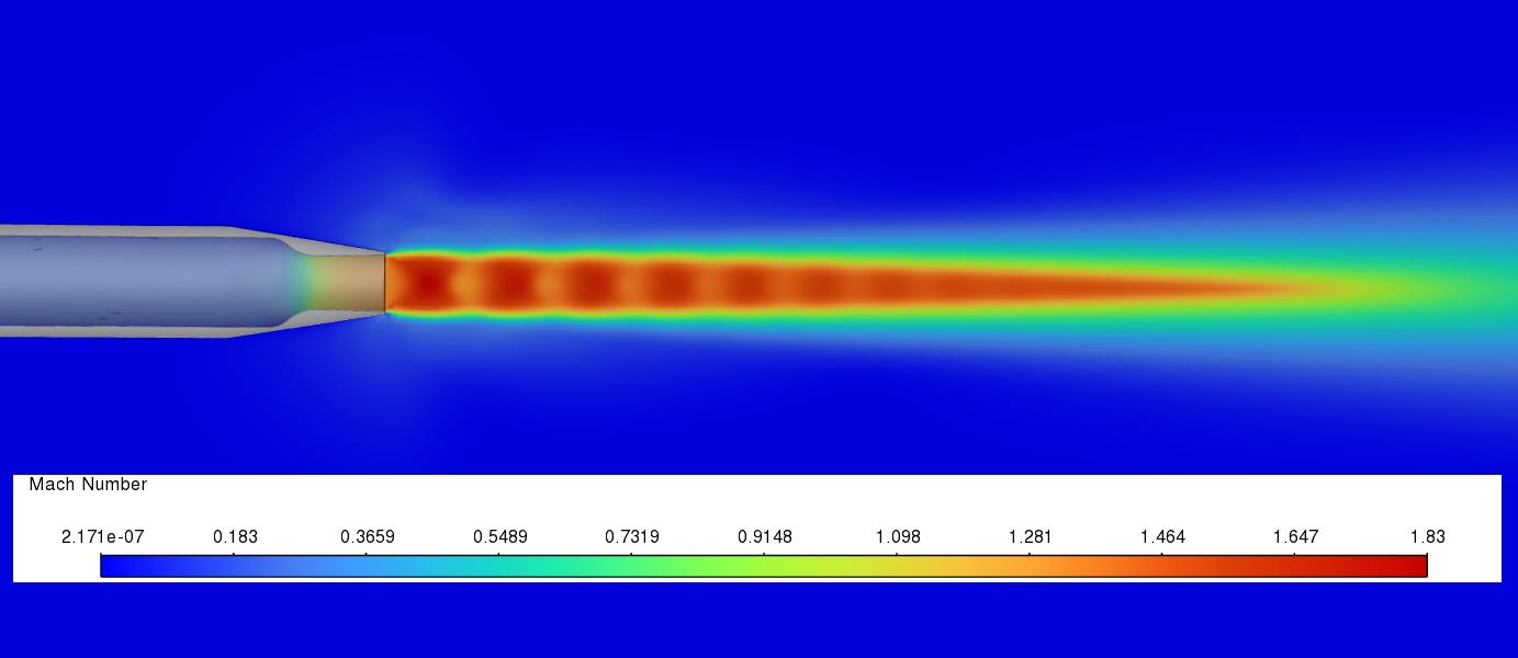
The insight: pressure based solver was able to provide adequate shock resolution with stable simulations, at a fraction of the computational resources.
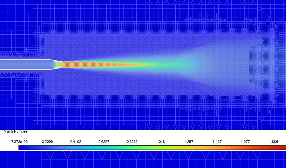
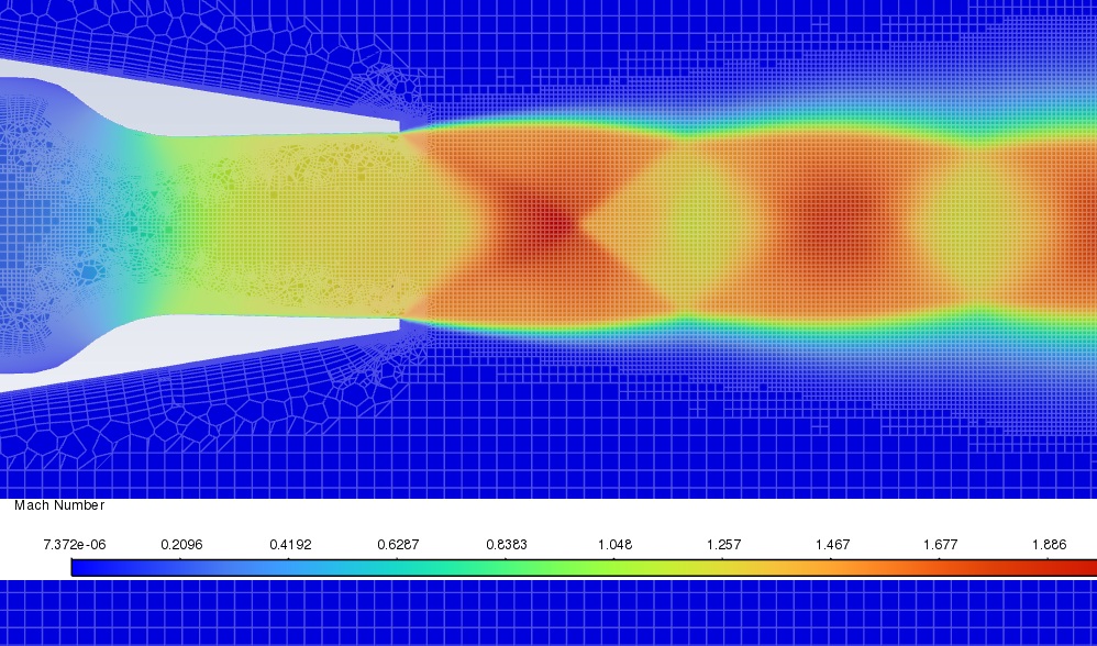
Mesh Adaption Without Runaway Cell Counts
The grid adaption methods available in Ansys Fluent are able to refine the mesh only in areas of interest, keeping mesh sizes low while improving solution accuracy.
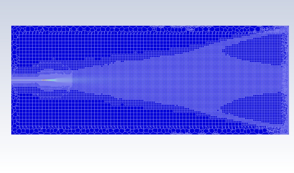
Manual Adaption: preview cells flagged by refinement parameter. For the test case, the density gradient metric served to refine only the shock train. The mesh grew from 4 M to ≈ 13 M cells and re-converged in < 100 extra iterations.
Automatic Adaption: Fluent’s automatic adaption every 100 iterations raised the mesh to ≈ 65 M cells but only refined where necessary, while also coarsening elsewhere, keeping memory manageable.
Choosing an error indicator:
- Density Gradient method is effective in refining shock regions, where changes in local density is rapid.
- Mach-Hessian method more effectively refines and coarsens the entire mesh, using the second derivative of local Mach number, to more effectively refine shear layers, and coarsen low-speed flow regions gradient method might miss.
Bottom line: mesh adaption is mandatory for sharp shocks but doesn’t have to significantly increase your cell count if you start coarse and refine selectively.
Practical Guidelines You Can Apply This Week
- Begin with a coarse mesh that resolves geometry features, not so fine as to cause long simulation runtimes; let the first run reveal where to adapt.
- Choose the pressure-based coupled solver as your default for mixed-Mach steady cases; use density-based only if solution stability or unsteady transients demand it.
- Use Mach-Hessian adaption when a more wholistic mesh treatment of the entire domain is desired.
- Apply local time stepping if initial simulations are unstable.
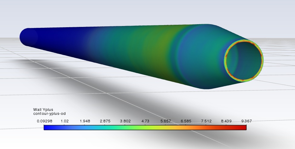
- Target y⁺ < 10 (not necessarily 1) when shock physics matter more than wall shear forces for mesh savings.
Expert Q&A Highlights
Q: Can I rely on pressure-based coupled for transient acoustic studies?
A: For weak shocks and broadband noise, yes. At strong shocks or large pressure fluctuations, the density-based explicit solver remains more robust.
Q: How does Fluent decide which cells to refine with Mach-Hessian?
A: It compares the second derivative of Mach number in each cell to the domain average. Cells above a user-set threshold split; you can cap the maximum cell count to prevent memory issues.
Q: What is the memory penalty of the Coupled algorithm compared to SIMPLE?
A: Each Coupled iteration uses slightly more RAM, but the quicker convergence means total memory-hours are often lower than with SIMPLE.
Conclusion: A Single, Faster Path to Clean Shock Diamonds
The old “pressure-based for subsonic, density-based for supersonic” rule is fading. Modern numerical methods let a pressure-based coupled solver tackle many transonic challenges, while mesh-adaption tools such as the Mach-Hessian indicator focus cells where they deliver the biggest accuracy jump. The result is cleaner shocks, leaner meshes, and far shorter turnaround, which is a winning trio for aerospace CFD teams facing tight budgets and timelines.
Need to see the workflows in action? Watch the full on-demand webinar for live solver demos, detailed mesh-adaption walk-throughs, and an extended Q&A with the engineer who ran the study. Or request a free consultation to get started on your simulation project today.