Nonlinearity in Ansys Mechanical for Beginners

Introduction to Nonlinearity Analysis

If you have ever run a simulation that felt like it should be straightforward, but the solver started taking tiny steps, repeating calculations, or refusing to finish, you have probably run into issues related to nonlinearity. Sometimes the model itself is perfectly reasonable, but the physics you are asking the solver to capture are more complex than a simple linear relationship. Nonlinearity is the umbrella term for situations where the response does not scale in a clean, proportional way as you increase load. That is why nonlinear analyses often require more solver effort, more careful setup, and more thoughtful interpretation of results.

This blog is part 1 of a two-part series on nonlinear analysis in Ansys Mechanical. In part 1, we will focus on what nonlinearity is and how to recognize where it is coming from in your model. We will walk through the most common sources of nonlinearity and use real-world examples to make each one intuitive. In part 2, we will discuss what convergence really means, how the solver works behind the scenes, and practical methods you can use to troubleshoot nonlinear convergence issues when they appear.

A useful way to understand nonlinearity is to compare it to linear behavior first. In a linear world, the relationship between load and response is proportional, meaning if you double the force, the displacement doubles. Stiffness stays constant, and a force versus displacement plot forms a straight line. In many real systems, stiffness is not constant. As you load a structure, it may become harder or easier to deform, or it may change behavior entirely. When that relationship curves instead of staying straight, the problem becomes nonlinear and the solver must work step by step, updating its idea of stiffness as the system changes. In Ansys Mechanical, nonlinear behavior most often comes from three sources: geometric effects, material behavior, and contact or status changes.

Geometric Nonlinearity

Geometric nonlinearity appears when the shape of the structure changes enough during loading that the shape change itself alters the result. If a part moves only a tiny amount, the load directions and internal force paths stay nearly the same as in the original model. But if the part rotates a lot, bends significantly, or stretches substantially, the directions of internal forces shift, lever arms change, and the structure begins to behave like it is in a new configuration. This can introduce nonlinearity even when the material remains perfectly elastic, simply because the geometry no longer resembles the starting shape.

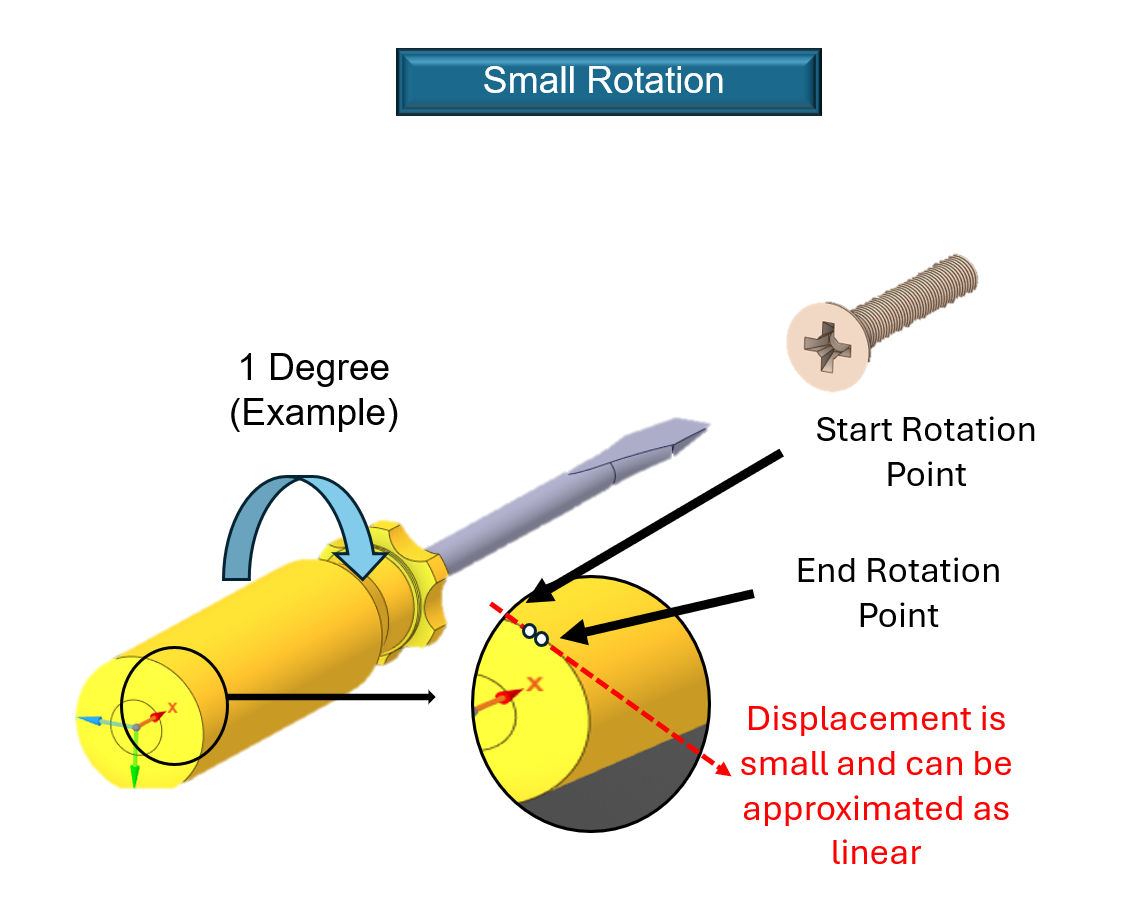
Example: Large Rotation

• Small Rotation: When you first start turning, you might twist the handle by just a fraction of a millimeter. In this tiny window, the ridges on the handle move in a way that looks like a straight line. Because the overall orientation of the screwdriver hasn’t changed, a structural simulation can use a “linear shortcut.” This assumes the force from your hand is acting on the exact same geometry it started with, which is a safe bet for microscopic movements.
• Large Rotation: Now, imagine you really crank the screwdriver, rotating it 90 degrees or more to drive the screw home. Every point on that handle is actually traveling along a curved, circular path around the shaft. If a computer model continues to use the straight-line “shortcut” for this large movement, it fails to realize the handle is following a circle.

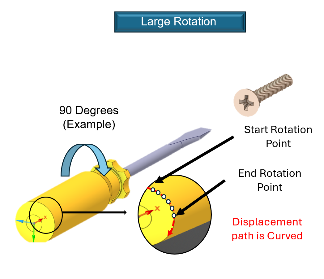
When a simulation ignores these curved paths, it results in a specific error called artificial radial growth. Because the mathematical shortcut calculates motion as a straight line tangent to the circle, it mistakenly predicts that the screwdriver handle is “flying” outward. In the software, the handle will appear to balloon in diameter or stretch away from the shaft simply because it is rotating. In the real world, a plastic or rubber handle doesn’t expand like a balloon just because you twist it; it stays the same size. By turning on the Large Deformation option in the Analysis Settings branch, the solver stops using straight-line shortcuts. Instead, it uses full trigonometric math to update the position of the handle at every degree of the turn. This ensures the simulation correctly tracks the curved motion, keeping the diameter of the screwdriver constant and providing an accurate look at the internal stresses without the “phantom” expansion caused by bad math.

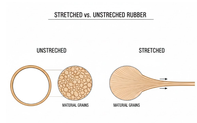
Example: Large Strain

Large strain becomes important when the deformation is no longer small in a mathematical sense, meaning the structure stretches or compresses enough that small strain assumptions no longer match reality. A simple real-world analogy is stretching a rubber band. A tiny stretch does not feel like it changes the rubber band much, but stretching it to twice its length clearly puts it into a very different configuration. In engineering structures, large strains can show up in thin membranes, seals, soft polymers, and any component designed to stretch significantly. When strains are large, both the strain measures and stiffness updates must reflect that the material points have moved far relative to each other. If this is ignored, the simulation may miscalculate the internal forces needed to reach a given displacement and may misrepresent the stress field because the underlying assumptions about deformation no longer apply.

Example: Stress Stiffening

Stress stiffening is one of the easiest geometric nonlinear effects to understand because many people have experienced it firsthand. A simple example is a guitar string. When the string is loose, you can pluck it from its resting position with very little effort and it moves a lot. When the string is tightened, doing the same thing feels noticeably harder and the string does not deflect as far. This happens because a tightened string already carries significant tension along its length. When you displace it, you are not only changing its shape, you are also forcing it to stretch slightly against that existing tension. Since the string is already loaded, even a small displacement immediately requires additional stretching work, so the string pushes back more strongly and behaves as if it is stiffer in that direction. In engineering, the same effect appears in cables, belts, membranes, thin shells, and pressurized structures, where preexisting stress changes how the structure responds to new loads. If stress stiffening is not included when it is important, the model can appear too flexible, natural frequencies can be predicted too low, and stability behavior that depends on the prestressed state can be missed.

Example: Spin Softening

Spin softening is most relevant to rotating machinery where rotation changes effective stiffness and stability. A simple way to think about it is to imagine a jump rope or flexible object being spun. As the rotation speed increases, the shape and tension distribution change, and the way the object resists bending or out-of-plane motion changes as well. In real rotating components like shafts, rotors, disks, and fans, centrifugal effects can stretch the structure and alter stress fields, while dynamic effects can reduce resistance to certain bending modes. The result is that rotation can effectively reduce stiffness in some directions, which can influence deflection patterns, vibration response, and critical speeds. If rotation driven stiffness changes are important to your design, they must be represented correctly or the simulation can miss key behavior.

Material Nonlinearity

Material nonlinearity appears when the material does not respond with a constant stiffness, meaning the stress strain relationship is not a single straight line. Even if the geometry changes are small and there is no contact, the material itself can create a nonlinear problem because its behavior depends on stress level, time, temperature, or prior loading. The most common material nonlinearities in mechanical simulation include plasticity, creep, and viscoelasticity.

Example: Plasticity

Plasticity is the classic example of a material changing behavior once it passes a limit. A simple everyday analogy is bending a paperclip. If you bend it slightly, it springs back because the deformation is elastic. If you bend it farther, it stays bent because permanent deformation has occurred. At the microscopic level, the internal structure of the metal rearranges in a way that cannot fully reverse when the load is removed. In structural components, plasticity appears in overload conditions, forming operations, highly stressed fasteners, regions near sharp corners where stress concentrations exist, and impact or crash events. Plasticity matters in simulation because it changes the stiffness once yielding begins and because it is path dependent. Two parts can reach the same final load but end up with different permanent deformation depending on how the load was applied and whether unloading happened along the way.

Example: Creep

Creep is time-dependent deformation under a sustained load, meaning that the part will continue to deform even when the applied load does not increase. An easy mental picture is a foam cushion under a heavy gym weight. The weight stays the same, but the cushion may slowly compress more over time. In metals, creep becomes especially important at elevated temperatures, such as turbine components, exhaust systems, and high temperature pressure equipment. In polymers, creep can occur at room temperature and can affect common items such as plastic clips, housings, and seals that slowly deform during service. Creep is nonlinear because time becomes part of the problem. The structure that looks acceptable at the beginning of the load history may become unacceptable later as strain accumulates, so the solver must step through time and track how the material evolves.

Example: Viscoelasticity

A fun and very clear way to understand viscoelastic behavior is to think about oobleck, a simple mixture of corn starch and water. If you gently dip your fingers into oobleck and move slowly, it flows and feels almost like a thick liquid. Your fingers sink in, and the material quietly moves out of the way. But if you slap it, punch it, or try to move your hand quickly, it suddenly feels solid and stiff, almost like you hit a firm surface. The material did not magically change into a different substance. What changed w as how fast you applied the force, and that loading rate changed how the internal structure resisted deformation. This is the key idea behind time dependent and rate dependent material behavior. Some materials respond differently depending on how quickly they are loaded. When the loading happens slowly, the material has time to rearrange internally and flow, so it appears softer and more compliant. When the loading happens quickly, the internal rearrangement cannot keep up, so the material resists motion more strongly and appears stiffer. In practical engineering terms, that means a component made of a polymer, rubber, adhesive, or damping material can behave one way under a slow steady load and a different way under a sudden impact, even if the peak force is the same. In simulation, this matters because you cannot describe the material with a single constant stiffness if the response depends on time or loading rate. To capture that behavior, the analysis must include time as part of the solution, and the material model needs data that defines how stiffness and deformation evolve with rate and over time.

Contact and Change of Status in Nonlinear Analysis

Contact nonlinearity appears when parts can touch, separate, and slide, creating varying load paths depending on contact state. If two parts are separated, they do not transfer force across any interface. When they touch, they begin transferring forces, which can suddenly increase stiffness and change how loads travel through the assembly. This “on” or “off” nature is fundamentally nonlinear and is one of the main reasons contact problems can be challenging.

Example: Unknown Contact Region

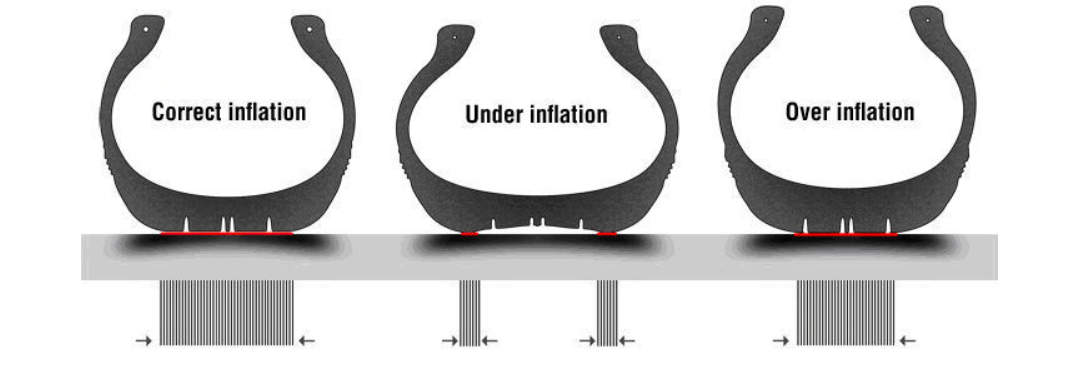
To visualize the complexity of an unknown contact region, imagine a vehicle tire resting on the ground. When the vehicle is empty, the tire touches the pavement over a relatively small, localized patch. However, as you add heavy cargo or passengers, the rubber compresses and deforms, causing the footprint to expand and the pressure distribution within that patch to shift significantly. You cannot predict the exact dimensions of this contact area ahead of time because the boundary of the footprint is determined entirely by how the tire reacts to the specific load applied. This becomes even more complex when considering tire pressure. A flat or under-inflated tire has a much larger, more irregular footprint that reaches toward the sidewalls, creating a broad but less stable contact area. Conversely, an over-inflated tire rounds out, making the contact region small and stiff, which focuses all the force into a narrow point.

In a mechanical simulation, this behavior is a primary source of nonlinearity. Just like the tire, surfaces in an assembly are often curved, slightly misaligned, or separated by tiny gaps that change as parts move. As a load increases, the true contact area can grow, migrate, or redistribute across the interface. The solver must constantly re-calculate where surfaces are touching and where they are apart, as every newly activated region of contact abruptly changes the overall stiffness of the model. Because these transitions can be sudden—moving from a gap to a hard stop in a single moment—the simulation must apply the load in small, controlled increments to prevent the mathematical solution from becoming unstable as the geometry of the contact area evolves.

Example: Friction and Sliding Behavior

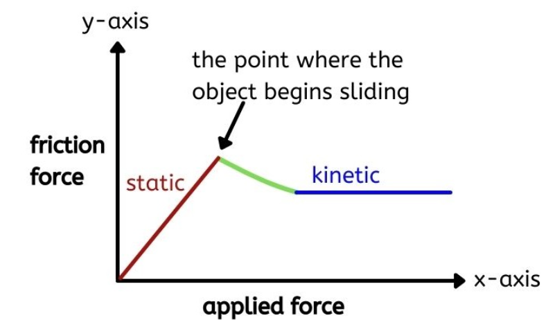
Friction adds another layer of complexity because it introduces a stick or slip transition that depends on history. Picture pushing a heavy box on the floor. At first, it may not move even though you are pushing. Then, once you push har d enough, it breaks loose and slides. Often it takes less force to keep it sliding than it took to start it. This happens because static friction can hold surfaces together up to a limit, then kinetic friction governs during sliding. In simulation, this matters because the solver must track which regions are sticking and which are sliding, and that status can change from one increment to the next depending on the prior solution. This makes frictional contact strongly path dependent and can significantly increase the difficulty of convergence.

Example: Change of Status Effects

To visualize change of status nonlinearity, imagine the behavior of a Newton’s cradle. In its resting state, the metal spheres are physically present but essentially “inactive” regarding the transfer of dynamic forces. In a simulation, this is similar to having elements that are part of the model but are not yet carrying any load, much like the middle spheres before they are struck. The moment the first sphere drops and impacts the row, a “change of status” occurs instantly as the middle spheres “turn on” to act as a bridge for the kinetic energy. This represents an abrupt shift in the load path where the system’s stiffness jumps from a series of independent hanging weights to a single, compressed unit.

This sudden activation is exactly what happens in structural simulations for staged construction or additive manufacturing. As a new 3D-printed layer is deposited or a support beam is bolted into a bridge, the material must be “activated” within the math to begin carrying its share of the stress. Because this change is binary (the part is either carrying load or it isn’t) the stiffness of the model changes in a jagged, non-smooth way rather than a gradual curve. These abrupt jumps are mathematically sensitive and require the solver to take very small, careful steps to ensure the sudden shift in the internal force path doesn’t cause the simulation to become unstable.

Nonlinear Analysis and Why Problems Need Special Treatment

Nonlinear analyses are not just harder because they are complicated. They are harder for very specific reasons. The solver must use an iterative approach to repeatedly adjust the solution until internal forces match external forces, and convergence is not guaranteed within the allowed number of iterations. Because stiffness changes during the solution, the solver often needs smaller increments and more iterations, which increases run time. Many nonlinear effects are path dependent, meaning how you apply the load changes the outcome, and superposition no longer applies, meaning you cannot solve separate load cases and add the results to get the combined answer.

A Practical Nonlinear Mindset Checklist

When you include any nonlinearity, be intentional about load ramps and stepping, especially for frictional contact and yielding materials. Expect small increments, because they are often how the solver safely follows real physics. Most importantly, remember that a converged solution is not automatically a correct solution. The setup, assumptions, and nonlinear options must match the real behavior you are trying to represent so the results are something you can confidently defend.