Ansys Workbench Mechanical | Modeling Buoyancy Load on Floating Structures
Modeling buoyancy load on a floating structure is possible in Ansys Workbench Mechanical if hydrostatic pressure is applied to submerged exterior faces. The FEA challenge is to determine how much of a body is below the surface, given the geometry, weight of the body, liquid displacement volume, and liquid density.
The depth to which a body sinks is not known in advance, so a series of load step solves is needed to find the depth and orientation of a floating body at equilibrium. The portion of the exterior surface that is below the surface changes with each load step, and applied pressures must be updated in a search for equilibrium.
Ansys SFFUN Command and Hydrostatic Input Arrays
The underlying Ansys solver can apply a spatial pressure gradient with various techniques, including the SFFUN command which uses for input an array containing hydrostatic pressures at surface node numbers, with the pressures calculated from node depth values. These pressures must be updated during SOLVE steps as a function of depth when a structure moves vertically in a liquid’s hydrostatic pressure “field” in large displacement analysis.
This article illustrates an Ansys Workbench Mechanical approach in which hydrostatic surface pressures are updated in a series of load steps, based on the depth of surface nodes as a structure bobs up and down.
Damping Application with ALPHAD Command in Ansys Mechanical
This simulation uses large displacement transient structural analysis, with damping applied via the ALPHAD command, in order to discover an equilibrium floating position and orientation of a structure.
The following example geometry was created in Ansys DesignModeler.
A hollow open-top tank was created in DesignModeler. Void interior space was filled with a second body representing air. The tank was assigned Structural Steel material, while the void interior was assigned the density and adiabatic bulk modulus of air, plus a zero Poisson’s ratio. Including “air” in the model aids calculation of the tank displacement volume.
Applying Hydrostatic Pressure with APDL Commands in Mechanical
The hydrostatic pressure is applied in an APDL Commands Object inserted at the Environment level of the Workbench Mechanical Outline. Vertex constraints prevent rigid body drifting in X and Z, and “yaw” rotation about Y.
Vertical movement in this model is in the global Y direction, with the liquid surface at Y=0. When meshing, element faces on exterior surfaces should be to be small enough to trace small changes in the position of the liquid surface. A coarser surface reduces final position accuracy.
More sophisticated modeling of complex floating objects could be considered by a rigid body approach within the CFD code CFX, or via fluid-structure interaction modeling with CFX and Ansys working together in the Workbench interface.
The present example seeks an equilibrium position using Workbench Mechanical alone, and does not consider liquid movements or the possibility of flooding interior spaces in a complex body.
Mass and Displacement Volume | Ansys Workbench
A preliminary small displacement static solve was performed with all degrees of freedom constrained, in order to calculate the total mass of the structure and the total displacement volume of the elements. This SOLVE is much quicker than the nonlinear transient analysis that will follow. These commands perform this static analysis:
fini
/solu
ANTYPE,0 ! static analysis
nlgeom,off ! small displacement
acel,0,0,0 ! no inertial load
allsel ! select full model
sfedele,all,all,all ! load removals
sfdele,all,all
fdele,all,all
bfedele,all,all
bfdele,all,all
!
esel,u,ename,,169,178 ! contact elements not wanted #####
d,all,all ! constrain all dof
irlf,-1 ! inertial relief ==> mass estimate
solve ! solve (quickly as possible?)
!
*get,my_mass,elem,,mtot,y ! get the mass active in Y
*get,cenx,elem,,mc,x ! centroid X
*get,ceny,elem,,mc,y ! centroid Y
*get,cenz,elem,,mc,z ! centroid Z
fini
!
! Discover volume of elements of this model
/post1
allsel
set,last
esel,u,ename,,169,178 ! Important: Unselect contact elements #####
etable,evol,volu ! volume of (remaining) elements
ssum
/com, .
/com, ####### SSUM RESULT ######
/com, .
*get,vol_of_elements,ssum,,ITEM,evol ! volume of all elements
Centroid Coordinates and Structural Displacement Volume
The above commands establish the mass of the structure, the centroid coordinates, and the displacement volume of the structure, including the body assigned “air” material properties. If the total volume is fully submerged, the calculated displacement volume produces a vertical force equal to the weight of displaced liquid. The purpose of the displacement volume is to calculate a reasonable mass damping value for the transient analysis.
The “air” material is very “soft”, so it does not significantly stiffen the structure. There are alternatives:
Convert air elements to MESH200 after assessment of displacement volume, with no need for contact pairs.
Assign “vol_of_elements” with the “Geometry” displacement volume, e.g.: vol_of_elements=1.8426e-3 ! Total displacement volume, this example
Volume in Details of “Geometry” must be calculated with all “air” bodies active, after which air bodies would be suppressed. In this example, Volume is 1.8426 litres, while Mass is 1.77 kg. If the model is submerged in water, Mass is less than 1.8426 kg of water displaced, so the body just floats if not flooded. If the Mass is too high, the body will sink.
Adding Damping to the Transient Analysis that Finds Equilibrium
This simplified buoyancy simulation does not include fluid elements. A hydrostatic pressure is placed on exterior nodes below the liquid free surface at Y=0.
A transient dynamic analysis with mass damping can find the equilibrium position, with the object settling down after a reasonable number of time steps. Mass damping can be applied by the ALPHAD command. The resulting damping matrix is proportional to the mass matrix.
Buoyant force on a floating object is a function of how far it sinks and so how much liquid it displaces. A “spring stiffness” for submersion is the slope of buoyant force versus depth travelled.
Approximating Stiffness in Ansys Mechanical | Buoyant Force
To approximate this “stiffness”, a “characteristic length”, “x”, has been calculated from the cube root of the “vol_of_elements” displacement volume calculated or entered above.
“Buoyant force” has been calculated from the product of displacement volume and a liquid density value entered by the user. “Stiffness” is calculated from F=k*x, where stiffness k=F/x, “buoyant force” of the submerged structure divided by “characteristic length”.
Given the mass of the structure and a “stiffness” estimate for the buoyant force, a critical damping value for a 1 degree-of-freedom mass subjected to a “spring stiffness” can be calculated for a body bobbing up and down when floating.
The critical damping value can be divided by the mass to find an argument for the ALPHAD command so that the floating body settles down quickly when it bobs up and down at the liquid surface during the transient.
Critical Damping and Un-Modeled Liquid in Buoyant Force
Below are commands that establish the argument for ALPHAD. A user must enter weight density (with correct units) of the un-modeled liquid providing the buoyant force.
The argument for ALPHAD is formed from a 1 DOF system consideration, in which we want to damp the floating body bobbing in the liquid. We divide a damping value (set here to 70% of critical damping) by the mass in order to get the ALPHAD argument.
liquid_weight_density=1000*9.8 ! Weight density of water for buoyancy <======
!
cube_root_vol=vol_of_elements**(1/3) ! characteristic linear dimension
!
! Characterstic stiffness of “bobbing” on the liquid surface
!
char_stiff=liquid_weight_density*vol_of_elements/cube_root_vol
!
! Characteristic time for one “bobbing” cycle if no damping
! period = 2*pi*sqrt(mass/stiffness)
!
time_period=2*3.14159*sqrt(my_mass/char_stiff) ! one “bobbing” cycle time
! Try 0.7*critical damping
! – Scale ALPHAD argument so that when multiplied by the mass matrix, we get a damping
! matrix that produces approximately 0.7*critical damping behavior.
!
my_alphad=0.7*(2*sqrt(my_mass*char_stiff))/my_mass ! Want C_matrix=alphad*M_matrix
!
ALPHAD,my_alphad ! want transient damping a bit below critical
!
TINTP,0.02 ! numerical damping; try to suppress “ringing” in structure
nstep=60 ! number of loadsteps (15 per undamped cycle in this test)
finaltime=time_period*4 ! 4 “bobbing” cycles (if not damped), characteristic dimensions
!
deltime=finaltime/nstep ! delta T for the time steps below
Because square and cube roots are taken, modest errors in displacement volume and mass have little effect on the damping coefficient. Taking 4 time periods of oscillation lets the “bobbing” movement damp out.
Hydrostatic Pressure Load Update and Time Integration
In Ansys, a Table Array can be formed to apply pressure to nodes as a function of depth. In this example, “vertical” is taken as the global Y value, with Y=0 taken as the position of the liquid surface:
*dim,mypress,table,3,1,,Y ! Table Array, pressure as fn of Y
mypress(1,0)=-100000,0,1 ! Depth positions in Y
mypress(1,1)=liquid_weight_density*100000,0,0 ! Pressure in TABLE ARRAY
! Using liquid weight density entered earlier
In this example, the above table array spans depths of up to 100000 meters, with the liquid surface at Y=0.
A numerical array is needed to store the original Y locations of exterior surface nodes in the mesh.
Column 1 of the array is filled with the original Y locations. Column 2 will be filled with the UY values of the nodes at the end of each load step. Column 3 will be filled with the sum of (Column 1) Y and (Column 2) UY at the end of each load step.
*get,maxnode,node,,num,max
*dim,mynode_y,array,maxnode,3 ! column 1 is original node Y
! column 2 will be node UY
! column 3 will be Y+UY for node
An array is needed to hold the pressure at each exterior surface node as a function of the depth values found in the above array:
*dim,mynode_press,array,maxnode
Vector operations are used to look up the pressures as a function of current node location, fill an array with these pressures, and apply them to surface nodes. This is done at the end of each load step, and these pressures are used during the next time transient load step. Note that the value of (Y+UY) is used to look up the hydrostatic pressure:
*vfill,mynode_press(1),ramp,0,0 ! Zero array content
! …other commands
*vitrp,mynode_press(1),mypress(1,1),mynode_y(1,3) ! pressure at current Y+UY
SFFUN,PRES,mynode_press(1) ! Pressures at nodes (per Y value)
sf,all,pres,1.0e-14 ! Small value added to above pressure as fn of current Y values
Time integration is performed by executing a series of SOLVE commands inside a loop. After each SOLVE, the hydrostatic pressures are changed to reflect the new surface node positions, with zero values employed above Y=0.
Time steps have to be small enough to maintain accuracy. The pressure profile is “out of date” at the end of a time step, so for accuracy, steps should not be too large. In the absence of any damping, the “bobbing” oscillations of the body will diverge when using this simplified time integration approach.
Since the objective here is only to find a static equilibrium position, time steps can be reasonably large if adequate damping is included. This example uses 15 time steps per undamped “bobbing” oscillation.
Workbench Mechanical Materials
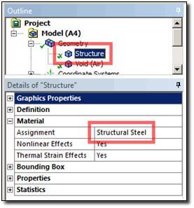
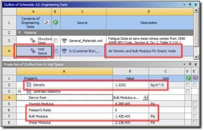
This example contains two bodies. The first called “Structure” is for the tank. “Structural Steel” has been assigned:
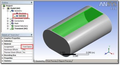
The second body “Void (Air)” is the empty space inside the tank, which has been filled by a body using DesignModeler. Material for this body has been set to “Void Space”, a material that was set to the bulk modulus and density of air, and a zero Poisson’s ratio. This Poisson’s ratio results in a shear modulus that is non-physical, but the values are so small that they will have no effect on most structures—if the stiffness was thought to be affecting the structure, a smaller bulk modulus could be entered, or Poisson’s Ratio could approach 0.5, or alternative methods for capturing the displacement volume of the empty voids in the model could be considered. The reason for including this “Void (Air)” body is to calculate the fluid Displacement Volume of the entire structure elements for calculation of a damping coefficient for the ALPHAD command. The “Void Space” can be observed in this image:
The following image shows properties of the “Void Space” material for air under adiabatic compression.
NOTE: An alternative is to make Poisson’s Ratio approach 0.5, for example 0.47, reducing Young’s Modulus and Shear Modulus to small values for the given Bulk Modulus. If Young’s Modulus and Shear Modulus become too small, gravity load can cause severe distortion, so Poisson’s Ratio for the “air” should not be set too close to 0.5.
In this example there is one contact pair, connecting “Void Space” to the structure. It has been set to Bonded, Asymmetric, Pure Penalty, a small Stiffness Factor, and a manual Pinball Radius. The “Contact Body” is air:
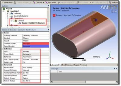
Users could consider a Multibody Part connecting the “Void Space” to the structure, and avoiding contact pairs, if the mesh consequences are satisfactory.
Wetted Surface
A Named Selection is used to indicate the External Hull for the purpose of this buoyancy floating analysis. It is set to all of the exterior faces of the model, including the external face of the “Void Space” material. If pressurized, the soft “air” material would severely distort, causing the solver to fail, warning the user if the solution produced a configuration in which the interior space could “flood”. This is not a guarantee that a real structure would not flood, but may catch some situations in which the structure could flood and potentially sink.
In the above image, note that all 8 external faces have been included in the Named Selection “External_Hull” including the exterior face of the “air” material in the void region. When the Commands Object that updates hydrostatic pressure is running, this Named Selection is assigned to a node component “n_external”:
cmsel,s,External_Hull ! select external hull nodes
cm,n_external,node ! remember external nodes as component “n_external”
This node component is selected when pressures are applied, so only user-chosen exterior surfaces are “wetted”. A mask is set to refer to exterior surface nodes:
*del,mymask,,nopr
*dim,mymask,array,maxnode
cmsel,s,n_external ! Nodes on model exterior
*vget,mymask(1),NODE,1,NSEL ! Fill masking array
Current Y-coordinate positions are calculated for these exterior nodes at each load step:
*vmask,mymask(1)
*vget,mynode_y(1,2),NODE,1,U,Y ! UY values of nodes on exterior
*vmask,mymask(1)
! Fill column 3 with updated Y+UY locations of nodes
*VOPER,mynode_y(1,3),mynode_y(1,1),ADD,mynode_y(1,2)
allsel
As mentioned, pressures are calculated for the current node Y positions in the third column of the mynode_y array:
*vfill,mynode_press(1),ramp,0,0 ! Zero array content
*vmask,mymask(1) ! Mask for surface nodes only
*vitrp,mynode_press(1),mypress(1,1),mynode_y(1,3) ! pressure at current Y+UY
SFFUN,PRES,mynode_press(1) ! Pressures at nodes per Y value
sf,all,pres,1.0e-14 ! Added to above pressure as fn of current Y values
The Transient Environment
The APDL Commands Object entered in this example first performs a static analysis with loads removed and degrees of freedom constrained, in order to find the displacement volume and mass, in order to set a damping coefficient for the ALPHAD command. It then executes a multiple load step transient analysis, in which the hydrostatic pressure load on the exterior nodes is updated at each load step according the depth below the liquid surface in the Y direction.
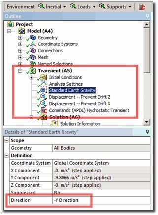
Gravity load is indicated by the user in a Standard Earth Gravity object. Note the –Y (negative) direction.
Enough displacement constraints are entered to prevent free translation in the X and Z directions, and free rotation (yaw) about the Y axis. These are not a necessity, but can make results review easier if the structure does not drift freely. The constrained vertices should be chosen so free rotation (pitch and roll) about X and Z can take place, free movement in the Y direction results, and the structure can undergo unrestrained thermal expansion or other distortions.
Vertex Displacements in Ansys | X & Z Direction
A total of 3 degree-of-freedom constraints will be sufficient. In this example, there are two vertex displacements in the Z direction, and one in the X direction. Although a remote displacement scoped to a face, edges, or a choice of vertices could accomplish this constraint, the use of a remote displacement creates extra elements, a pilot node, and can greatly increase the wavefront of a model, causing a longer solution time. Working with 3 constraints on vertices will generally be preferred. In some models, a remote point might be intentionally used to measure structure rotation at equilibrium.
If the liquid surface is to be located at global Y=0, then the geometry needs to be in an initial position in which the open “air” void faces are not below the liquid surface. In addition, the structure should not be located in a starting location so far above the liquid surface that the structure drops below the surface and floods the open “air” void faces.
An ideal starting location is near the equilibrium position. With complex geometries, the structure may undergo substantial pitch and roll while approaching equilibrium. Yaw may be zero if rotation about the vertical Y axis is prevented by displacement constraints, but pitch and roll should not be prevented by constraints.
The APDL Commands Object used in this example is listed in the Appendix at the end of this document.
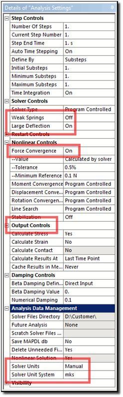
Analysis Settings for the Transient Environment
The details for Analysis Settings are relatively simple. Real control of the solution of the model will be exercised by the APDL commands in the APDL Commands Object that is inserted in the Transient Environment.
The “Number of Steps” can be left as is, since the Commands Object will control time stepping. Note that Time Integration is On.
“Weak springs” should Off in case there are large movements.
“Large Deflection” is On since the model moves a significant distance in comparison to its dimensions, and may rotate significantly.
“Nonlinear Controls” might be left as-is, or be tweaked by a user.
“Output Controls” should be considered, since the structural transient can generate a substantial amount of results data over a large number of substeps. (GBytes of data can easily result.)
“Solver Units” can be set to the units employed in the APDL Commands Object for the setting of the parameter liquid_weight_density. Users may find that this is most easily done in SI units, because of the peculiarities that result in other systems of units, such as Newtons per cubic millimetre. Note that Weight Density is Mass Density multiplied by acceleration due to gravity.
Users should ensure that the solution is performed in the units assumed in the APDL Commands Object. “Solver Units” can help to ensure that this is done.
The Mesh
Mesh density must satisfy a number of criteria. It needs to be fine enough to give an accurate structural solution. A coarser mesh may return adequate structure displacement values, but high accuracy stresses will require a finer mesh, particularly in regions of interest.
Mesh density on the exterior will affect the accuracy of the final position when floating in a liquid. Interested users could perform a sensitivity analysis on the effect of modified external face mesh density.
In the image below, the “Void Space” material is colored orange. A viewing setting like this helps to identify the regions in the model that model empty space, but are considered to be interior spaces that affect displacement volume. The empty interior of the hull of a ship would be typical of this “Void Space”.
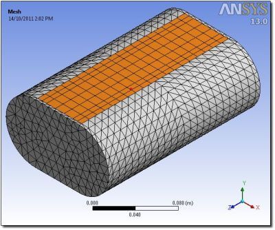
Users should be careful to set the soft “Void Space” material as the Contact in a bonded contact pair, and to set it to asymmetric contact. The “Void Space” can be meshed with low-order elements and a relatively coarse mesh, to reduce model size and solution time.
Results
Vertical movement by the structure can be observed in a plot of Y-displacement Max and Min values versus time:
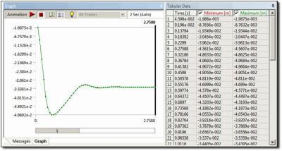
Note that the “bobbing” motion of the floating object has settled down by the end of the transient.
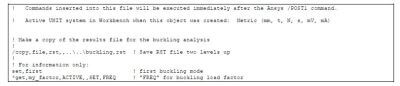
A postprocessing APDL Commands Object can be used to plot the final pressure profile on the model, for example:
! Plot pressure arrows at the end of the last time step
set,last ! Load last result
!
/plopts,info,3 ! Legend controls
/show,png ! Generate a PNG image file
/gfile,600 ! Pixel height at line border
!
/view,1,1,1,1 ! Isometric view
/psf,pres,norm,2 ! Show Normal Pressure Arrows
nplo ! Plot of nodes
eplo ! Plot of elements
/view,1,0,0,1 ! End View
nplo ! Plot of nodes
eplo ! Plot of elements
!
/view,1,1,1,1 ! Isometric view
/psf,pres,norm,3 ! Show Normal Pressure Contours
nplo ! Plot of nodes
eplo ! Plot of elements
/view,1,0,0,1 ! End View
nplo ! Plot of nodes
eplo ! Plot of elements
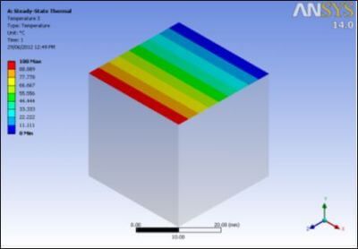
This is a plot of the pressure profile for the final near-equilibrium position of the mesh. Note that black and white colors have been reversed—this color reversal can be done by additional APDL commands. The pressure at the top of the object can be observed to be virtually zero. Note that the value is not exactly zero because the node pressures assigned by the SFFUN command must be followed by an SF command with a very small non-zero value.
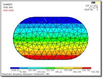
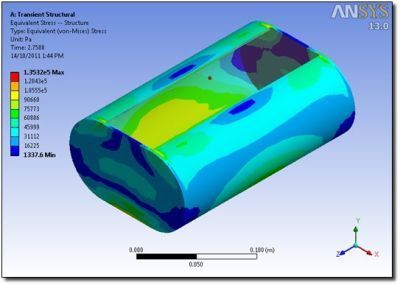
Stresses at the end of the transient may be of interest in some models.

Summary
Using Ansys Workbench Mechanical to simulate buoyancy loads on a floating body has been illustrated. In the approach presented, a hydrostatic pressure load is applied to a Named Selection of exterior nodes that are located below a liquid surface. A transient structural simulation is run by looping through many load step solves, with the surface pressure load recalculated for each load step. The load steps must be short with respect to the “bobbing” frequency of the floating object at the liquid surface. Artificial damping is employed via the ALPHAD command of Ansys, using a damping coefficient that is about 70% of critical damping for the body “bobbing” on the liquid surface. User inputs are limited to the liquid weight density, and placing the initial position of the body. The simulation damps body movements, determining an equilibrium position and orientation for the floating body.
A variety of simplifications were included in this example:
- It is assumed that no liquid leaks inside the closed hull, and that any interior spaces are filled with zero density very soft elements to capture total displacement volume. It is assumed that exposed faces of the “Void Space” elements will not be pressurized when the structure position changes.
- Bodies of complex shape could have more than one floating equilibrium position. Resulting orientation depends on initial conditions, and is influenced by mesh density, time step size, and damping. In this simulation, damping was chosen to get the body to quickly stop bobbing up and down at the surface.
- The damping level used here may be much higher than what is encountered in typical liquids like water. The objective of the present approach is to quickly determine one equilibrium position.
- It is assumed that there is sufficient buoyancy for the object to float. The body is assumed not to leak. If the body will not float, it will drift downward at a terminal velocity dictated by the applied ALPHAD damping value, until the end of the transient simulation is reached, or until “Void Space” elements distort severely.
Convergence on the nonlinear deformations of a flexible structure will automatically be considered by the large displacement setting employed in the analysis, however the changing displacement volume is not considered in the damping calculation, so damping may diverge from near-critical in extreme cases. Accuracy may require a larger number of substeps. Full load is instantaneously applied with the KBC,1 command, not ramped up, so smaller time steps may be desired with nonlinear body buckling deformations. The analysis could be considered “quasi-static”, and enough structural damping should be used to prevent “ringing” vibrations of the body during the simulation. In the present example, the TINTP command is used to try to reduce vibration of the structure during the transient.
The present example considers the vertical bobbing up and down of a floating model. Such an object could also pitch, yaw and roll on the liquid surface. The length of the transient simulation when rotation of the structure is significant may need to be considered. The ALPHAD damping value was chosen to suppress vertical bobbing of the floating body. A transient will need to run long enough to damp out any rotational motions, too. Lower settings of the damping value with a longer transient might be considered if a rolling motion is expected to re-orient the body.
The position and orientation solution for a complex floating body may be path dependent, and may depend on initial conditions of location, orientation and velocity. The approach presented here uses a large damping value in an attempt to find an equilibrium position. Neutral stability, and the degree of stability in the final orientation are not considered—the applied damping simply stops motions. Users may want to do further simulations after the initial “stable” floating position is established, and see whether small perturbations will cause body rolling when ALPHAD damping is reduced to much smaller values. The UPCOORD command might make the at rest floating position become the initial condition for a separate analysis of stability.
Appendix – Input File for Hydrostatic Pressure and Simulation Control
Here is the APDL Commands Object that applies a pressure profile, sets a liquid weight density value, finds mass plus a value for the floating “stiffness” of the “bobbing” motion of the floating body, sets an ALPHAD damping coefficient, and approximates how long to run the simulation to approach an equilibrium position. It then performs the transient simulation through a series of short time steps, updating the pressure profile at each time step according to depth of the surface nodes during time steps of the analysis.
Note that a user must update the liquid weight density setting in the code below according to the liquid, and may want to adjust other settings according the particular model that is being considered. Correct use of units must be observed in setting liquid weight density. In addition, mass density of materials must exist in all material properties of the model to be analyzed. Gravity loading comes from the Workbench Mechanical model.
! Commands inserted into this file will be executed just prior to the Ansys SOLVE command.
! These commands may supersede command settings set by Workbench.
! Active UNIT system in Workbench when this object was created: Metric (m, kg, N, s, V, A)
! ##################################################
! Hydrostatic Pressure on a Floating Structure in a Liquid
!
! This example uses Void bodies (density and bulk modulus of air) to include interior spaces.
! Pressure load as function of depth.
! Loop to find equilibrium position, using transient.
!
! Note: – All of the model is selected for analysis
! – All of exterior nodes are “wetted” if they fall below Y=0
!
! Note: – Too few substeps causes inaccuracy.
! – Transient too short causes inaccuracy.
! – Element faces too large causes inaccuracy.
! – Damping stabilizes, but affects path-dependent orientation.
!
! NOTE: It is assumed that “ringing” frequencies of the structure are much higher than the
! frequency of “bobbing” of the floating structure on the liquid surface.
! If this is not the case, then much longer transients may need to be studied, with
! much lower damping settings used in the ALPHAD and TINTP commands below.
!
! Warning: This demonstration input file has had only limited testing.
! Use at your own risk.
!
fini
save,temporary_db_here__,db,,model
*del,all ! delete parameters
*del,all,_PRM
*del,,PRM_
!
!
! USER MUST DEFINE LIQUID WEIGHT DENSITY HERE <<<<<<<<<<<<<<<<<<<<<<<
! USER MUST DEFINE LIQUID WEIGHT DENSITY HERE <<<<<<<<<<<<<<<<<<<<<<<
!
liquid_weight_density=1000*9.8 ! Weight density of water for buoyancy <========
! Newtons per Cubic Meter <========
! Use correct units! <========
!
!
!
!
! Discover the mass of the model and a characteristic “bobbing” stiffness
!
fini
/solu
ANTYPE,0 ! static analysis
nlgeom,off ! small displacement
acel,0,0,0 ! no inertial load
allsel ! select full model
sfedele,all,all,all ! load removals
sfdele,all,all
fdele,all,all
bfedele,all,all
bfdele,all,all
!
esel,u,ename,,169,178 ! contact elements not wanted #####
d,all,all ! constrain all dof
irlf,-1 ! inertial relief ==> mass estimate
solve ! solve (quickly as possible?)
!
*get,my_mass,elem,,mtot,y ! get the mass active in Y
*get,cenx,elem,,mc,x ! centroid X
*get,ceny,elem,,mc,y ! centroid Y
*get,cenz,elem,,mc,z ! centroid Z
fini
!
! Discover volume of elements of this model
!
/post1
allsel
set,last
esel,u,ename,,169,178 ! Important: Unselect contact elements #####
etable,evol,volu ! volume of (remaining) elements
! pretab,evol
ssum
/com, .
/com, ####### SSUM RESULT ######
/com, .
*get,vol_of_elements,ssum,,ITEM,evol ! volume of all elements
/com, .
cube_root_vol=vol_of_elements**(1/3) ! characteristic linear dimension
!
! Characterstic stiffness of “bobbing” on the liquid surface
!
char_stiff=liquid_weight_density*vol_of_elements/cube_root_vol
!
! Characteristic time for one “bobbing” cycle if no damping
! period = 2*pi*sqrt(mass/stiffness)
!
time_period=2*3.14159*sqrt(my_mass/char_stiff) ! one “bobbing” cycle time
!
fini
!
parsav,scalar,my_temporary_parameters,txt
resume,temporary_db_here__,db
parres,change,my_temporary_parameters,txt
!
/delete,my_temporary_parameters,txt ! clean up
/delete,temporary_db_here__,db
/delete,my_temporary_parameters,txt
!
allsel ! select full model
cmsel,s,External_Hull ! select external hull nodes
cm,n_external,node ! remember external nodes as component “n_external”
allsel
!
!
!
*del,mypress,,nopr
*dim,mypress,table,3,1,,Y ! Table Array, pressure as fn of Y
!
*get,maxnode,node,,num,max
*del,mynode_press,,nopr ! array to hold pressure at each surface node
*del,mynode_y,,nopr ! array to hold current node Y value
*dim,mynode_press,array,maxnode
*dim,mynode_y,array,maxnode,3 ! column 1 is original node Y
! column 2 will be node UY
! column 3 will be Y+UY for node
*del,mymask,,nopr
*dim,mymask,array,maxnode
cmsel,s,n_external ! Nodes on model exterior
*vget,mymask(1),NODE,1,NSEL ! Fill masking array
*vget,mynode_y(1,1),node,1,loc,Y ! Fill column 1 with node Y location
*vget,mynode_y(1,3),node,1,loc,Y ! Fill column 3 with node Y location
!
allsel
!
mypress(1,0)=-10000,0,1 ! Depth positions in Y
mypress(1,1)=liquid_weight_density*10000,0,0 ! Pressure in TABLE ARRAY
! Using liquid density
!
! Loop through time steps (load steps) in transient analysis:
!
fini
!
/SOLU
!
ANTYPE,4 ! time transient analysis
TRNOPT,FULL
LUMPM,ON ! Lumped mass matrix for… speed?
!
NLGEOM,1
NSUBST,1,0,0 ! 1 substeps in each load step
AUTOTS,0
!
! Gravity from Workbench Mechanical Environment <<<<<<<<<<<<<<<<<<<<<
!
kbc,1 ! Do NOT ramp up loading, rely on damping below.
! Ramping exaggerates oscillation divergence.
! Ramp loading only if significant structure deformation.
! Want damping, ideally related to mass, displacement
! volume, and liquid density.
! Want ~ 0.7* critical damping for “bobbing” movement.
! Recall 1 DOF System critical damping = 2*sqrt(m*k).
! Using ALPHAD setting for mass damping.
!
! Try 0.7*critical damping
! – Scale ALPHAD argument so that when multiplied by the mass matrix, we get a damping
! matrix that produces approximately 0.7*critical damping behavior.
!
my_alphad=0.7*(2*sqrt(my_mass*char_stiff))/my_mass ! Want C_matrix=alphad*M_matrix
!
ALPHAD,my_alphad ! want transient damping a bit below critical
!
TINTP,0.02 ! numerical damping; try to suppress “ringing” in structure
nstep=60 ! number of loadsteps (15 per undamped cycle in this test)
finaltime=time_period*4 ! 4 “bobbing” cycles (if not damped), characteristic dimensions
!
deltime=finaltime/nstep ! delta T for the time steps below
!
allsel
!
!
!
!
! Transient solves inside the following loop
!
*do,ii,1,nstep
TIME,ii*deltime
!
cmsel,s,n_external ! Nodes on model exterior
!
*vfill,mynode_press(1),ramp,0,0 ! Zero array content
*vmask,mymask(1) ! Mask for surface nodes only
*vitrp,mynode_press(1),mypress(1,1),mynode_y(1,3) ! pressure at current Y+UY
SFFUN,PRES,mynode_press(1) ! Pressures at nodes per Y value
sf,all,pres,1.0e-14 ! Added to above pressure as fn of current Y values
allsel
!
*if,ii,lt,nstep,then
!
SOLVE ! take one load step in time
!
! Update mynode_y second column values (UY values)
*vmask,mymask(1)
*vget,mynode_y(1,2),NODE,1,U,Y ! UY values of nodes on exterior
*vmask,mymask(1)
! Fill column 3 with updated Y+UY locations of nodes
*VOPER,mynode_y(1,3),mynode_y(1,1),ADD,mynode_y(1,2)
allsel
*endif
*enddo
! Return control for final SOLVE in Ansys, which follows this line
The body should be observed to be at rest by the end of the simulation, otherwise a longer transient should be simulated by increasing the value of the parameter “finaltime” in the above code.
Don’t Hesitate to Ask for Advanced CFD Modeling Support
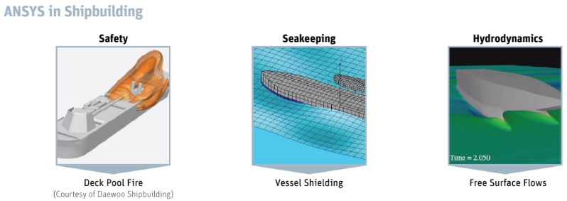
The volume of fluid approach brings up new possibilities for sophisticated modeling, which calls for more preparation on the part of the CFD engineer.
The volume fraction requires new boundary conditions that change with vertical position. Keep hydrostatic pressure in mind. The meshing method became increasingly intricate, necessitating further improvements at the free surface transition.
While we recommend Ansys Fluent, some CFD analysis software toolkit will be required for post-processing to see the free surface. Volume of fluid (VOF), in short, is difficult to define. This is why we strongly recommend seeking advice from engineering experts for expensive projects which require computational accuracy and swift execution.