HFSS Cable Modeling Workflow | Bundles, Harnesses & W-Element Export

Cable modeling is a beta feature that enables modeling of a cable and harness and their EM solution in HFSS. The workflow allows creating straight wires and twisted pair cables and furthermore supports creating bundles of individual cable assemblies. The cable bundle jacket modeling options include insulation as well as braided shied. The final cable assembly can also be exported as a W-element for subsequent transient and frequency domain simulations in Ansys Circuit. This document provides a summary of cable modeling workflow in HFSS.

1. Getting Started with HFSS Cable Modeling:

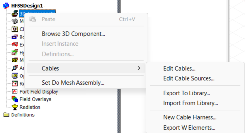
The Cable modeling workflow (with the beta feature enabled) is accessible through 3D Components in HFSS Project Manager. As shown in Figure 1, right-click on 3D Components and select Cables, the menu provides access to new and existing cable models, modifying cable sources, export to and import from cable library, modeling cable harness and exporting cable models as W-elements.

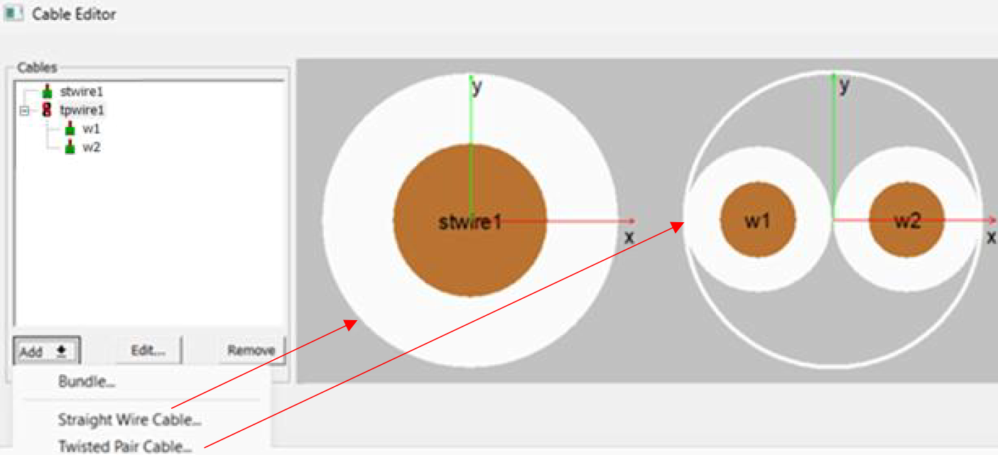
To model a new cable bundle, select Edit Cables, add a Straight Wire Cable first which can then be used to create Twisted Pair Cable. Either of the AWG and ISO standards can be chosen to model single wire with insulation type and material being the other design options. Once a single, straight wire is defined, a twisted pair can be modeled from the single wire definition with the desired turns per meter or lay length. Multiple straight wires can be added and twisted pair cables be created out of a unique, straight wire definition or multiple twisted pairs can use the same wire. Figure 2 shows cross sectional views of a straight and twisted pair cable.

2. Cable Bundle:

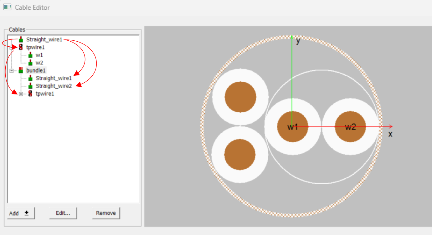
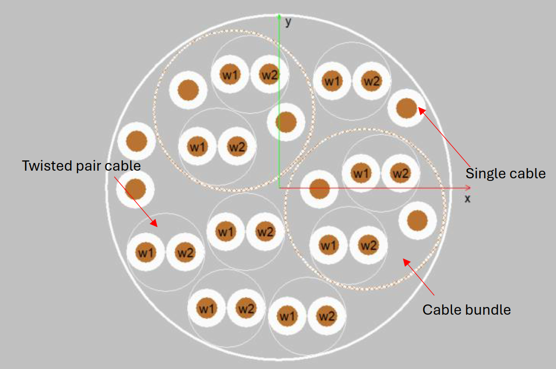
Once the individual cables are defined, a cable bundle can be created comprising any number of straight wires or twisted pair cables. Under the Add option, select Bundle. The individual cables (straight wire/ twisted pair) can be added into the bundle definition such that the bundle cross-section can automatically adjust with “AutoPack option checked” or manually defined by setting the inner diameter of the jacket. Manual definition of the bundle size allows adjustments in the relative positions of the individual cables. Furthermore the outer jacket of the bundle can be chosen appropriately from insulation, braided shield or no-jacket types. In case of braided shield jacket, the Shielding tab additionally incorporates various parameters associated with the shield design. Figure 3 shows a cable bundle “bundle1” comprising a pair of straight wires and a twisted pair cable. The cable editor supports hierarchy, which enables infinite nesting of bundles within bundles. The workflow automatically generates the cross sections based on a list of constituent cables and bundles without the need to draw complicated geometries as depicted in Figure 4.

3. Cable Path and Harness Design:

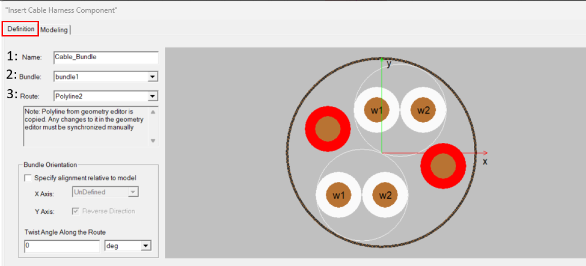
After the cable bundle is set up, the next step is to define the cable routing path by defining a polyline in HFSS. With the cable bundle (cross section) and the trajectory defined, the final step in cable modeling is creating the cable harness. In the Cable menu shown in Figure 1, select New Cable Harness which opens the dialog shown in Figure 5, assign a name, select the bundle and polyline to complete the harness definition. The alignment of the harness model relative to the bundle definition can be set by defining the orientation vector, and Twist Angle controls the harness twisting along the route by selecting units of degrees, degree minutes, degree seconds, or radians.

4. Cable Excitation/Termination:

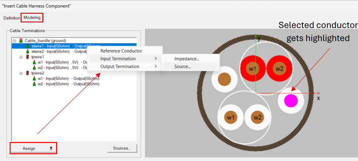
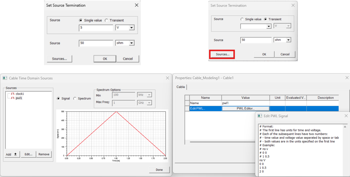
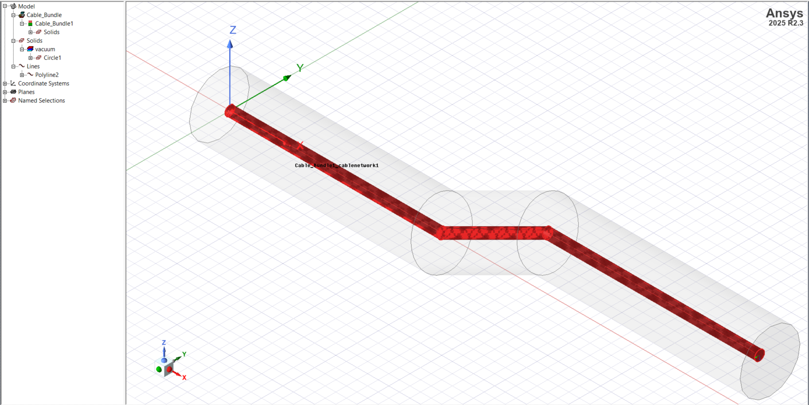
Once the cable assembly is defined, the next step is to assign reference ground to the cable harness and source and termination to the individual cables.  If the braided shield is defined, that acts as a Reference Conductor by default. However, if the bundle jacket type is not a braided shield, one of the constituent conductors must be defined as a reference conductor which gets labeled as “ground” in the Cable Terminations list. In the Modeling tab, select a conductor wire, either from the list of Cable Terminations, or right click on the graphic, and then select the appropriate option as shown in Figure 6. Selecting Source opens the Set Source Termination dialog as depicted in Figure 7. Either a single value source may be used to excite a cable, or transient waveform can be defined as a Clock signal or Piecewise Linear signal. Selecting either signal opens the appropriate dialog to assign the desired parameters and shows the signal graphed as time domain signal or frequency spectrum. The PWL Editor also allows defining custom source waveforms as per the example format in the editor window as shown in Figure 7. Similarly, the inputs and outputs of all other cables in the harness definition can be terminated with a source or impedance. In the end, the 3D model of the cable harness is created as a red cylindrical object representing the cable harness and the cylinder’s axis corresponding to the polyline as shown in Figure 8.

5. Cable Simulation:

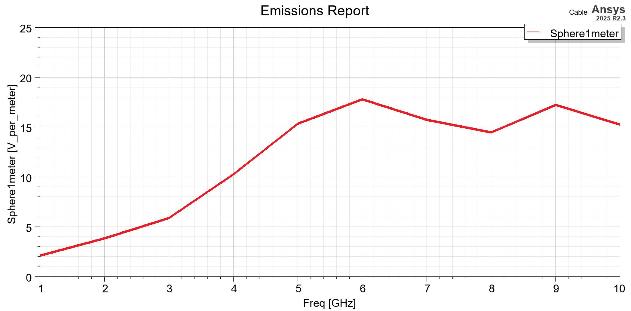
The harness is listed as a PEC material in the History Tree. The PEC designation is only used to have the Solve Inside option cleared within HFSS for the object’s volume. The cable’s 3D component definitions control the actual conductor and insulator materials, geometry, and other cable parameters. These definitions are the basis of 2D Extractor and Circuit simulations that occur in the background when the HFSS analyses is performed. Additionally, based on the source’s assignment in the harness definition, an excitation “Cable_Bundle1_cablenetwork1” is automatically created and listed in the Project Manager. An airbox is finally modeled that fully encloses the cable and allows fields computation outside the cable trajectory e.g., a cylindrical airbox is shown in Figure 8. After solving the model, field results from the cable can be overlaid on the airbox. In the end, define an Analysis setup and frequency sweep to extract EM field distributions for the cable harness. For +5v source excitation on “tpwire1” in Figure 6, a sample E-field distribution and emissions report is shown in Figure 9.

6. Cable Harness W-element:

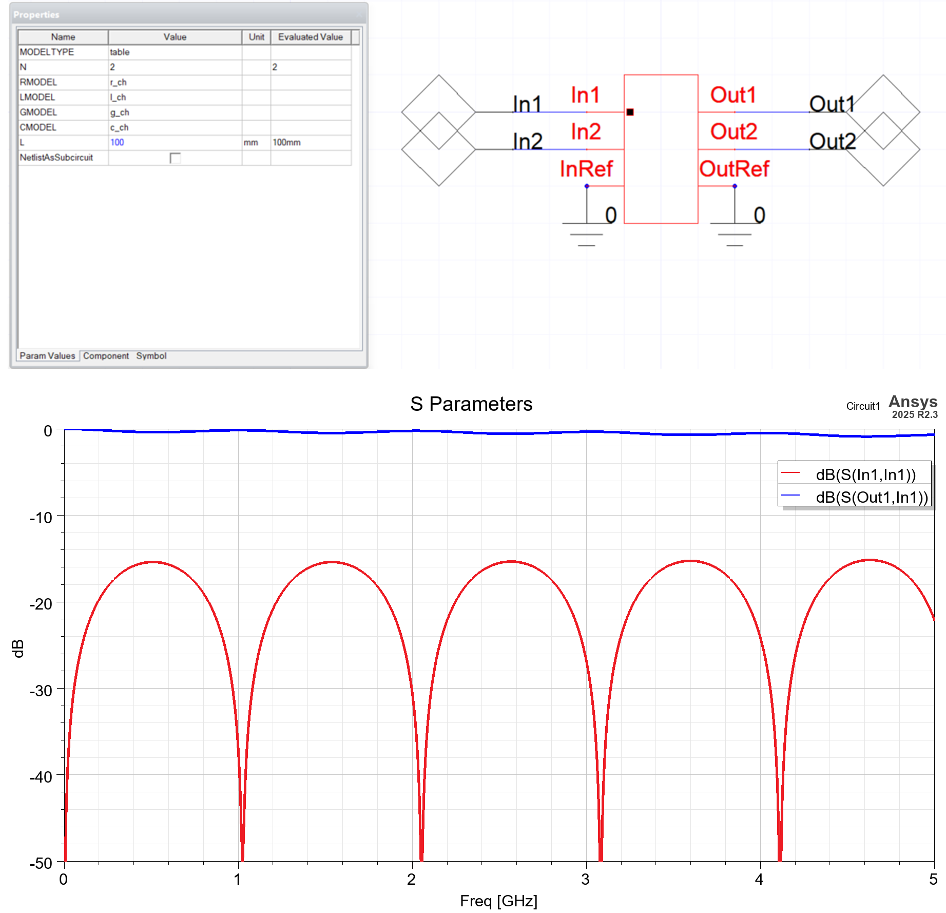
A W-element model is a distributed model for transmission lines used in HSPICE-compatible circuit simulations. It captures all material properties like skin depth, conductive and dielectric losses, characteristic impedance, transmission loss and mutual coupling. In HFSS cable workflow, W-element for a cable is calculated based on cross-section of the harness and contains a port for each source defined in the harness definition. In the Cable menu, select Export W-Elements and enter the maximum frequency for RLGC extraction. An HSPICE file is created as “cable harness name_welems.sp” in the design results folder in which RLGC values can be read via notepad or any other text editor. Figure 10 shows the W-element model of the cable harness and its properties. The variable “L” defines the length of the cable being simulated in AEDT Circuit.

HFSS Cable Modeling in Summary:

A comprehensive overview of the HFSS cable modeling workflow is summarized which does not require explicit modeling of complex cable geometries. The routing path can be modeled via polylines, and flexible source definition enables emissions calculation at various distances from the cable. Furthermore, W-element export allows linear network analysis or transient simulations of the overall cable assembly.

Need help validating your cable harness models?
Our electromagnetic simulation experts can help you implement HFSS cable workflows, optimize harness layouts, and export accurate W-element models for system-level analysis. Explore EMI/EMI Consulting services or talk with an HFSS Specialist →