This is Part 2 of a series on transient impact analysis in Ansys Mechanical. Part 1 established methods for determining analysis duration and time-step sizing when a flexible rod impacts a rigid surface. Part 2 extends the study to a flexible-on-flexible scenario: a cylindrical rod impacting a thin plate, in which both components deform during the event.
Summary of the Flexible-on-Flexible Impact Problem
In Part 1 of this series, we described how to determine the analysis duration and the number of time steps required to achieve accurate transient structural analysis results simulating the impact of a flexible cylindrical rod on a rigid surface, and how to verify compliance with various hand calculations based on energy methods.
Part 2 of this series focuses on the same geometry while it impacts another, more flexible object. In this case, being a flat plate. We explore further how to define the transient structural duration and the number of time-steps based on the flexibility of both components, and discuss how we can expect results to change depending on whether we choose to establish our time-step sizing based on the more rigid or the more flexible of these two components. Read below to better understand these topics and more.
Model Setup: Calculating Plate Stiffness for Transient Impact Analysis
In Part 1, we began with our first example, which explored the impact of a cylindrical bar on a hard surface. The bar had a diameter of 25.4 mm, a length of 254 mm, and a mass density of 7.85e-06 [kg/mm³]. This bar was dropped from 1 meter from the bottom face.
The second model we use in Part 2 contains our shaft geometry, but now, instead of impacting a rigid surface, it impacts a more flexible plate. The impacted plate is 254x254mm and is 5mm thick. It is made from the same material as the shaft, and the shaft’s bottom face is in contact with the plate’s top face. We need to calculate the plate’s stiffness in the impact direction. To do this, we will simply support all edges of the plate and apply a 9.9079 N load at the top of the shaft, then calculate the maximum deflection of the plate.
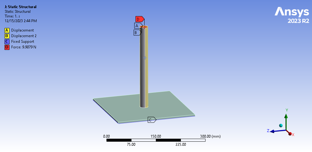
Figure 1: Cylindrical Rod and Flat Plate Geometry
The deflections are as follows:
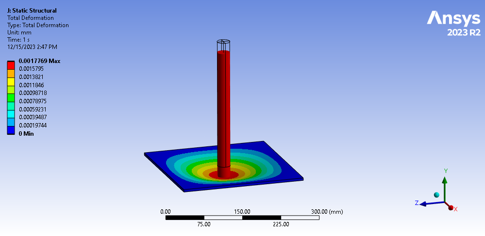
Figure 2: Static Structural Deflection Results
Specifically, we want the average Y-direction deflection on the plate immediately under the rod.
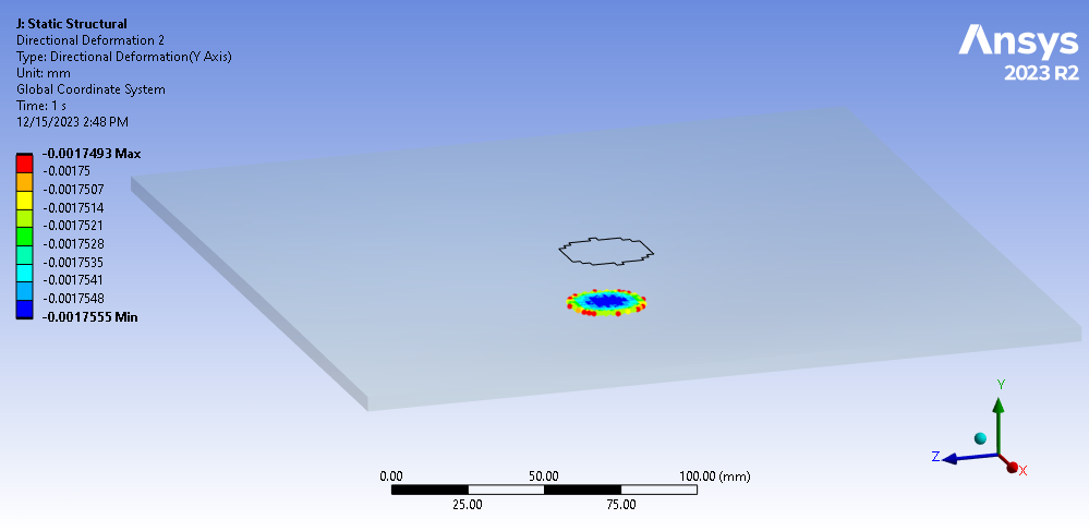
Figure 3: Deflection Results of Nodes Below Rod on Plate
Ansys Mechanical provides this average directly from the Details of this result, and this average equals -1.7533e-003 mm. Therefore, the directional stiffness of our plate is:
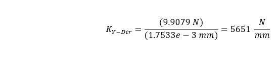
This value is significantly lower than that of the shaft, and it is expected to dictate the duration of the impact period.
Modal Analysis to Determine Impact Duration
When performing a modal analysis, one should keep in mind that at the time of impact, the mass of the plate will be combined with the mass of the cylinder; therefore, the modal analysis must consider both components, which yields the following results.
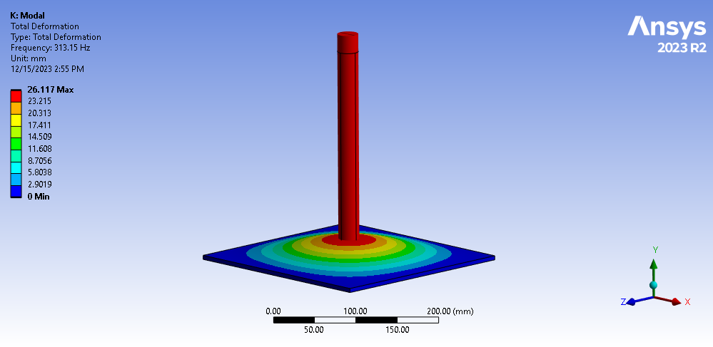
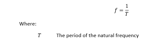
Figure 4: Modal Analysis Results of Combined Plate and Cylindrical Rod Model
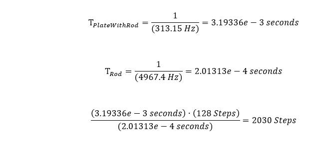
With the natural frequency calculated at 313 Hz for the mode shape aligned to the impact direction, the period of the transient analysis can be calculated as follows:

We know from Part 1 of this series, that we can expect accurate assessment of both deflections and stresses if we consider 128 time steps during the solution… but this is based on the period associated with the natural frequency of the bar. The period associated with the plate’s natural frequency is much longer. Can we expect to achieve the same quality of results if we consider this number of time steps for this longer period? Let’s see.
Running the Transient Impact Analysis with 128 Time Steps
We define surface contact between the bottom faces of the bar and the top face of the plate and impose the 4428 mm/sec velocity on the bar as an initial condition, as we calculated in Part 1 of this series, representing a drop of our bar from a distance of 1 m before impacting our plate.
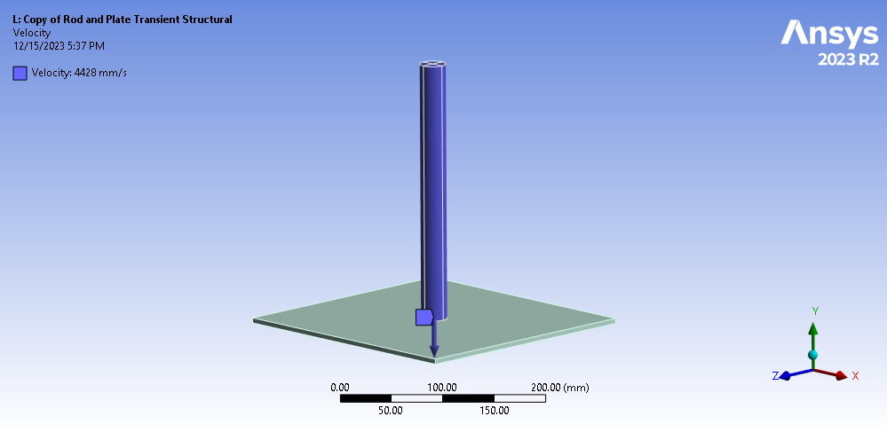
Figure 5: Transient Structural Model with Initial Velocities Applied to Cylindrical Rod
Running our transient structural analysis shows the instant at which maximum deflections occur in the plate while impacted by the cylindrical bar.
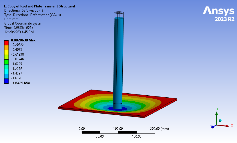
Figure 6: Maximum Deflections from Transient Structural Analysis While Considering 128 Time-Steps
If these deflections are plotted over time, they will appear as follows:
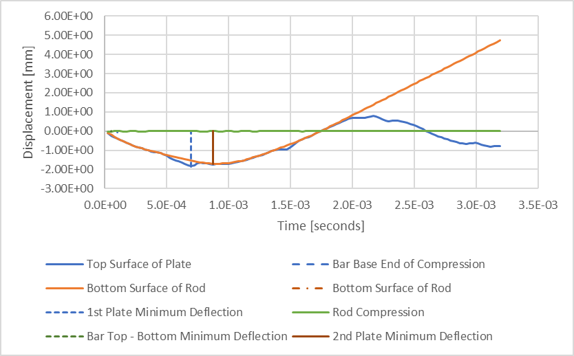
Figure 7: Deflections Plotted Versus Time While Considering 128 Time-Steps
Here we see the bottom surface of the rod (orange) has a gentle parabolic shape, while the top surface of the plate (blue) has a more complex response and seems to be bouncing with the bottom of the rod during impact. The green line represents the compression of the rod, which seems very small (-0.03187 mm) relative to the deflection of the plate (-1.8159 mm). Plotting only this rod’s compression verifies these observations.
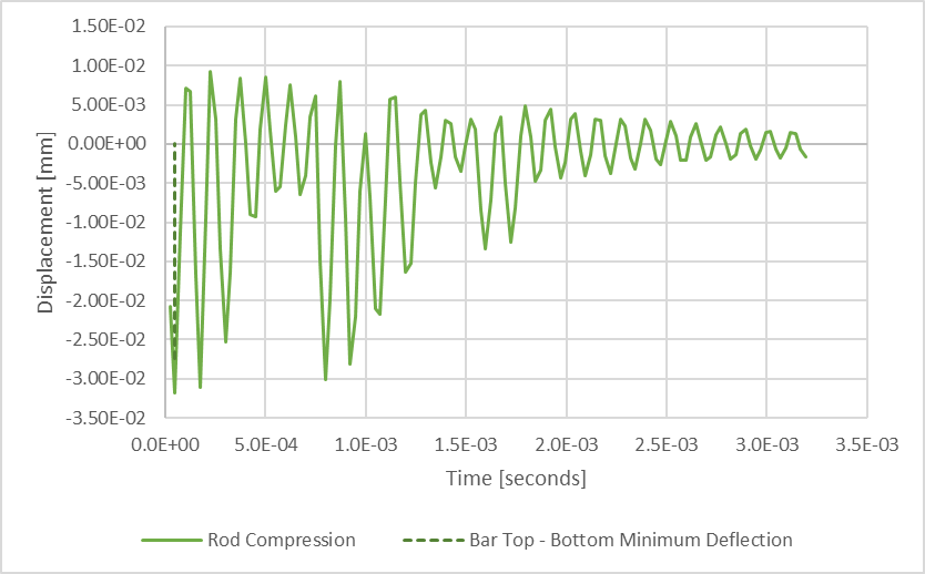
Figure 8: Rod Compression Plotted Versus Time While Considering 128 Time-Steps
It should be obvious that using 128 time steps resolved the plate deflections very well, but the rod compression response may be underrepresented at this capture rate.
Increasing to 1015 Time Steps for Higher-Fidelity Rod Response
If we consider the rod’s natural frequency to determine the capture rate, we might expect to require 2030 time steps for this duration.
Changing analysis settings to use 2030 time steps instead of 128 means the analysis will likely take 16 times longer to solve and generate proportionally larger result files as well. To reduce the cost of our hunch, let’s instead consider half as many time steps, which suggests 64 time steps per rod natural frequency period and will solve in half the time. Therefore, reanalyzing the same model with 1015 time steps yields the following results.
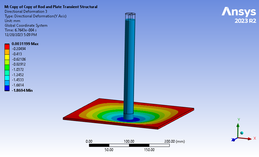
Figure 9: Maximum Deflections from Transient Structural Analysis While Considering 1015 Time-Steps
With a maximum deflection of 1.8694 mm, these results are only 1.4% larger than those obtained with 128 time steps. Plotting these deflections vs. time shows greater resolution of the plate’s dynamic response as it bounces against the bottom of the rod during the rod’s parabolic deflection path.
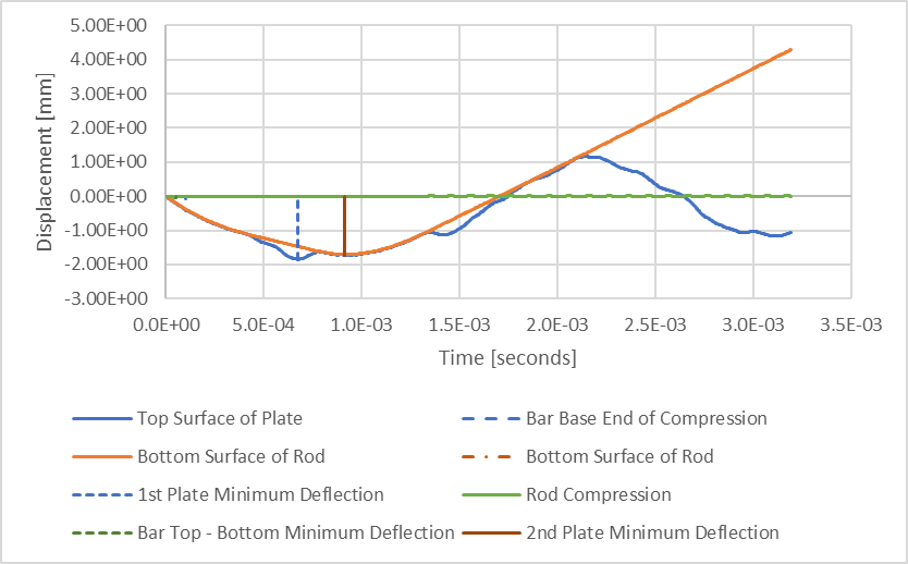
Figure 10: Deflections Plotted Versus Time While Considering 1015 Time-Steps
Closer examination of the rod compression shows much better resolution while considering 1015 Time-Steps.
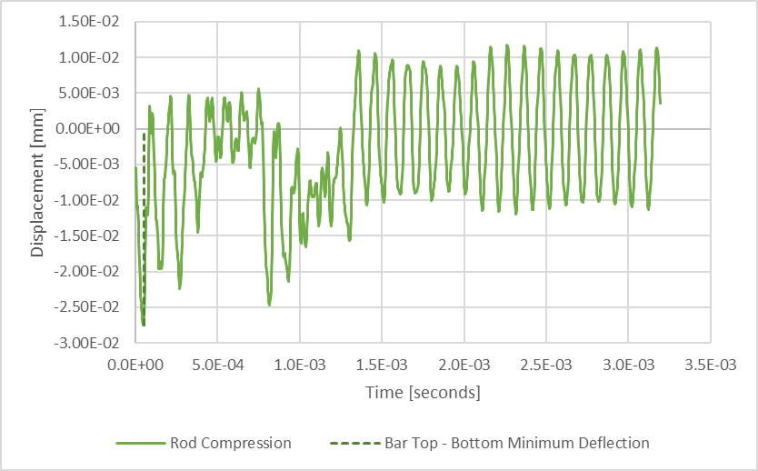
Figure 11: Rod Compression Plotted Versus Time While Considering 1015 Time-Steps
When More Time-Steps Are Worth the Computational Cost
Is this analysis effort justified if we only achieve a 1.4% change in the maximum deflection magnitude of the plate? The answer will relate to where the results of interest are. If our goal is to understand the plate’s deflections, then 128 time steps will be sufficient. Conversely, if we are interested in the rod’s response as it impacts our plate, we will need to adjust the time step to accommodate the rod’s dynamics, which would suggest 1015 time steps or more for this particular scenario. But there is more we can learn from this comparison.
Examining our deflection plots, we see that the maximum plate deflections are indicated by a dashed blue vertical line, which occurs earlier than the maximum downward displacement of the rod’s bottom surface. We have identified a 1.4% difference in these displacement results when comparing the 1015-time-step analysis to the 128-time-step analysis. If we focus on the plate’s maximum deflections near the rod’s bottom-surface maximum downward displacements, we find that the displacement difference between the two analyses is within 0.5%.
| Number of Time Steps | Bottom Surface of Rod Displacement [mm] | Top Surface of Plate Deflection [mm] |
| 128 | 1.7134 | 1.7357 |
| 1015 | 1.6981 | 1.7264 |
Figure 12: Table Listing Maximum Deflections Per Part
Based on these observations, we can establish that if our goal is to understand the general deflections of our softer component (plate) in our impact problem, we can achieve adequate results with only 128 time-steps and still uncover important details of that component’s more complex dynamic response. If our focus is to better understand this complex dynamic response, we can use additional time steps, but recognize that the response may not differ significantly.
Validating Results Against Hand Calculations
Let’s compare our finite element deflection results to our hand calculation by equating the potential energy of our falling cylinder with the elastic energy of our flat plate.
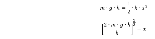
In this case, we will need to ensure proper units:

Therefore, our theoretical maximum deflection of the plate should be about 1.87 mm, but our analyses show 1.74 mm at 128 time steps and 1.73 mm at 1015 time steps, which are differences of 7.3% and 7.8%, respectively.
If we consider the maximum downward deflection of the plate at any time during the event, we find 1.82 mm at 128 time steps and 1.85 mm at 1015 time steps, a difference of 3% and 1.4%, respectively. However, I am not inclined to think that our hand calculation accounts for the complex vibrational response of two flexible bodies, and therefore, I focus more on the former comparison than on the latter.
Verifying Impact Duration Against Natural Frequency
As a final check, we can measure the time associated with the impact in these two scenarios, i.e., the time it takes for the plate surface to reach its original position. The duration of impact is reflective of ½ the period of its natural frequency in the direction of compression. Therefore, the following should be true.
Therefore:
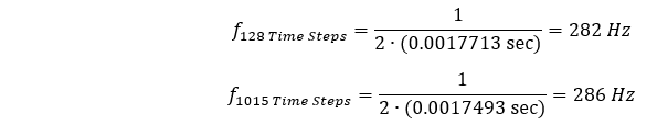
By either measure (282 or 286 Hz), we are about 9% different from the expected impact duration associated with our estimated impact frequency of 313.15 Hz. These results show that our method for estimating the duration of the impact event and its associated capture rate remains reasonable, but less precise as we include additional flexible participants in the event.
Stress Results: 128 vs 1015 Time Steps in Transient Impact Analysis
Of course, we crave to view the dynamic stress results, which appear as follows:
{% video_player “embed_player” overrideable=False, type=’hsvideo2′, hide_playlist=True, viral_sharing=False, embed_button=False, autoplay=False, hidden_controls=False, loop=False, muted=False, full_width=False, width=’828′, height=’518′, player_id=’151506240519′, style=” %}
Figure 13: Animation of Transient Structural Impact Stresses While Considering 128 Time-Steps
{% video_player “embed_player” overrideable=False, type=’hsvideo2′, hide_playlist=True, viral_sharing=False, embed_button=False, autoplay=False, hidden_controls=False, loop=False, muted=False, full_width=False, width=’828′, height=’518′, player_id=’151504073256′, style=” %}
Figure 14: Animation of Transient Structural Impact Stresses While Considering 1015 Time-Steps
Plotting these maximum stresses over time for both time-stepping schemes illustrates how these peak stresses differ.
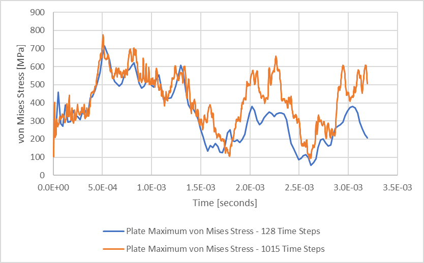
Figure 15: Maximum Plate von Mises Stress Plotted Versus Time
The general trend of peak stress is captured while using 128 time steps for our event, but the 1015 time-steps reveal higher frequency oscillations, which are filtered from the analysis using fewer time steps. In either case, the peak stress is 714 MPa with 128 time steps and 776 MPa with 1015 time steps.
Key Takeaways for Transient Impact Analysis Time-Step Selection
While exploring the transient analysis of the impact of a cylindrical rod on a more flexible plate, we confirm that our method for determining the analysis duration based on the natural frequency of the more flexible of the two components is satisfactory. Also, we confirm that using 128 time steps over this duration still yields maximum deflection results within 7.8% of those from classical hand calculations based on energy equations. We did find that we could produce more detailed results by solving with more time steps, but at the expense of longer analysis times and larger result files. The difference in maximum deflections was only 1.4%, and the difference in maximum stress was under 8% while considering 1015 time steps instead of 128.
Part 3 of this series will consider our cylindrical rod as it impacts another cylindrical rod of the same stiffness, thereby completing our understanding of the analysis settings for event duration and time-step size in transient structural analyses.
Working on transient impact analysis or time-step convergence studies? SimuTech Group’s FEA consulting engineers work with Ansys Mechanical across linear, nonlinear, and transient structural workflows. For more on explicit dynamics, see our article on Ansys LS-DYNA for car crash simulations. Learn more about Ansys Mechanical or contact us to discuss your project.