Applying Spatially Varying Data in Ansys Mechanical with APDL

Why Use APDL?

When modeling a real-world scenario, it is often necessary to define spatially varying properties that come from external sources, such as a separate analysis model or test measurement data. APDL in Ansys Mechanical can help extend standard workflows when external data needs to be interpolated and applied to properties that are not directly supported by built-in imported load tools.

Mechanical has robust capabilities for mapping external load data to an analysis model through the External Data component in Workbench and the Imported Load analysis component in Mechanical. While this approach is automated and useful, it is limited in the types of properties it can define. With a few APDL commands, external data can be interpolated and applied to a wider range of properties, including interface properties.

Potential applications of this approach include:

• Contact thermal conductance based on pressure from a structural analysis
• Contact friction coefficients that vary based on position or temperature
• Contact stiffness values that vary based on position

This article explains the APDL concepts required, shows example syntax, and provides practical tips for implementing APDL in Ansys Mechanical for spatially varying interface-property workflows.

Process Overview

The process of applying external data as an interface property has two major steps:

1. Interpolate the external data into a rectangular grid of points and format as an APDL TABLE
2. Apply this TABLE to the correct interface real constant set for the contact elements

What is an APDL TABLE?

In APDL, a TABLE is a special type of numeric array that behaves like a function rather than a simple list of values. Instead of being indexed only by integers (1, 2, 3, …), TABLE indices can be real-valued and represent physical quantities such as X, Y, Z, time, or temperature.

When the solver requests a value at an index that does not exactly match a table entry, APDL performs linear interpolation between the nearest index values. This is what makes TABLEs ideal for describing spatially varying properties.

The table’s axis values (the independent variables) are stored in the ‘0th row’ and ‘0th column’ of the table. The property values are stored in the interior cells (1…IMAX, 1…JMAX). Once defined correctly, the TABLE can act as a function that looks up property values for a given set of independent variables (such as coordinates), interpolating as necessary.

The following syntax shows how a TABLE may be declared in APDL:

*DIM,my_field,TABLE,nx,ny,1,label_x,label_y

Values in a TABLE are accessed or assigned using parentheses. Depending on context, the values inside the parentheses can represent real-valued axis locations (lookup with interpolation) or integer cell indices (direct assignment).

my_field(x,y) = value

See this resource for details on this command: *DIM

Step 1: Interpolate external data and create TABLE

Most external datasets arrive as scattered points with a list of (X, Y, Z) locations and a measured or computed value at each location. An APDL TABLE, however, requires values on a structured grid (a rectangular lattice of points on a plane or rectilinear 3D domain). Therefore, it is necessary to convert the scattered input into a grid of points. This can be done in APDL using the *MOPER command, which includes a MAP operation to interpolate source values at target locations and store the result in a new array. The following is example syntax for this command:

*MOPER,result_array,target_points,MAP,source_values,source_points

The MAP operation stores results in a numeric array, which then needs to be converted to a TABLE so it can be used as a lookup for interface properties. This can be done by declaring a TABLE with the appropriate size (using *DIM) and then populating the TABLE using loops (*DO…*ENDDO). Note that the indices of the TABLE (the 0th row and 0th column) must be populated with the X and Y coordinates of the target grid points. The interior cells of the TABLE are then populated with the interpolated values, starting at row and column 1.

Refer to the following resource for details of this command: *MOPER

Step 2: Apply TABLE to interface properties

Once the TABLE is defined, the second step is connecting it to the interface definition used by the solver.

In APDL, many interface behaviors are controlled through real constants, especially for contact elements and special-purpose interface elements used in Ansys Mechanical. Workbench typically creates one or more real constant sets behind the scenes and assigns them to the contact/target element types.

Real constant sets can be modified using the RMODIF command, which has syntax as follows:

*RMODIF,NSET,STLOC,V1

NSET is the real constant set ID. In Mechanical, these commands should be made part of a command snippet that is part of a contact object in the model tree. In that case, NSET can be set to cid or tid. This is because Workbench will inject the commands of a command snippet into the analysis input file (ds.dat) at a location determined by where it sits in the Mechanical tree. When the command snippet is attached to a contact object, the command snippet is injected immediately after the commands that define the contact. In the ds.dat file for each contact there are lines that assign numerical values to the cid parameter for the interface contact elements and to the tid parameter for interface target elements. So, using cid or tid is simply referencing parameters that have already been defined.

STLOC is the location of the real constant to be modified. The correlation between location number and property is element specific. The documentation for each element type includes a table describing what each real constant controls. For 3D surface-to-surface contact generated by Mechanical, the contact element type is commonly CONTA174. For that element type, real constant 14 defines thermal contact conductance, real constant 3 defines the normal penalty stiffness factor, etc.

Finally, it is possible to substitute a TABLE for the real constant value by enclosing the table name in % characters. This tells MAPDL to evaluate the real constant from the table (interpolating as necessary). The final APDL commands look like:

*RMODIF,cid,14,%my_table% – for setting thermal contact conductance for contact elements

*RMODIF,tid,14,%my_table% – for setting thermal contact conductance for target elements

See this resource for more information on the command: *RMODIF

Use this link to see the complete real constant table for CONTA174: CONTA174 – Real Constants

Other Implementation Steps for APDL in Ansys Mechanical

Exporting contact data from Mechanical

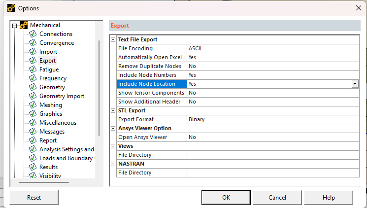
Exporting contact data from Mechanical for use in another analysis can be done from within the Mechanical GUI. As an example, contact pressure can be exported by defining a contact tool. In the right-click menu there is an option to export the results to a .csv file.

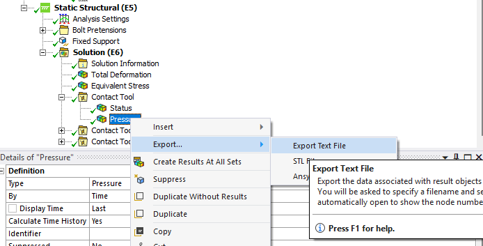
Note that by default only the node ids and result value are exported. To export the nodal coordinates, an additional option from within Mechanical options must be checked.

Reading CSV Files into APDL

When using APDL in Ansys Mechanical, engineers can read external data in multiple ways. Two common approaches are:

– *TREAD: reads delimited text (including CSV) directly into a TABLE parameter.

– *VREAD: reads fixed-format text into numeric arrays and requires a FORTRAN-style format statement.

A typical workflow is to read CSV into a TABLE with *TREAD (for convenience), then copy the numeric values into a standard ARRAY for calculations and interpolation. This is why you often see a TABLE-to-ARRAY copy step prior to mapping.

Practical Limits of This APDL Workflow

This approach is powerful, but there are practical limits to keep in mind:

• Memory can be a concern for TABLEs with many grid points. 2D tables are more efficient for memory but require that all your grid points lie on the same plane. 3D tables could be used but the number of grid points can grow rapidly.
• If the solver queries outside the table’s defined range, behavior depends on the consuming element. Build tables that cover the full region the solver will query.
• Mapping only works if your source coordinates match the solver coordinate system. Be explicit about global vs local coordinate systems.

Example Workflow

The following steps constitute an example workflow that could be used to apply thermal contact conductance values to a steady state thermal analysis based on pressure result from a static structural analysis:

1. Export pressure results from the static structural analysis to a CSV file
2. Convert pressure to thermal contact conductance values based on material data. This could be done in a spreadsheet or scripting language like Python.
3. Export thermal conductance values and nodal coordinates to a CSV file
4. Create APDL command based on the explanations above to read in the thermal conductance values, interpolate to a TABLE and apply the table to real constants sets for contact and target elements
5. Add APDL commands to appropriate contact object in thermal analysis

A project archive is available for an example problem that applies spatially varying thermal contact conductance values to a contact in Ansys Mechanical. The archive includes the thermal conductance values in a CSV file located in the project’s user files directory, along with APDL commands in a command object beneath the contact in the Mechanical model tree. This example provides a practical reference for implementing the technique in a real-world workflow.

Download the spatially varying TCC example project

APDL in Ansys Mechanical: In Conclusion

Applying spatially varying properties with APDL in Ansys Mechanical can be challenging when the required data comes from external sources or needs to be assigned to interface properties not directly supported through standard imported load workflows. By using APDL commands, engineers can interpolate external data into a TABLE, apply it to contact real constant sets, and extend Mechanical’s capabilities for more advanced simulation scenarios.

This approach can be especially useful for workflows involving contact thermal conductance, position- or temperature-dependent friction, contact stiffness, and other interface behaviors that vary across a model.

Need help extending your Ansys Mechanical workflow? Connect with SimuTech Group to learn how our simulation experts can help you apply APDL, automate advanced setup tasks, and build more flexible workflows for complex engineering analyses.