Mesh-Independent Result Extraction Using Volume Averaging with Ansys DPF

Published: 08/06/2026

Updated: 08/06/2026

1. Volume Averaging with Ansys DPF: Study Objective

The primary objective of this study is to introduce and validate the concept of Volume Averaging for element-based finite element analysis (FEA) output quantities (such as von Mises stress, equivalent plastic strain or even individual stress or strain components).

When extracting regional or macroscopic data from an FE model, standard arithmetic averaging introduces a severe geometric bias if the mesh density is non-uniform. This study demonstrates how volume averaging mathematically minimizes mesh-induced bias, ensuring that extracted results reflect true physical states rather than mesh dependent variations in the model. Furthermore, this report outlines a practical approach to implementing this methodology via automated Python post-processing script using the Ansys Data Processing Framework (DPF), utilizing the Ansys result file (.rst).

2. Significance of Volume Averaging

In FEA, displacements are calculated at the nodes and stress/strain results are computed at the integration points within each element. As elemental fields are computed at each element, stress/strain discontinuities are seen across the element boundaries; a coarse mesh displays severe discontinuities compared to a fine mesh which minimizes them.

A simple averaging of stress values of a group of elements or for the whole model is calculated as below:

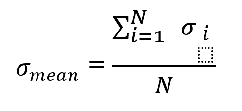
where σ_i is the stress of element i (could also be extended to element i and integration points) and N is the number of elements. A simple averaging introduces numerical bias whenever the mesh is non-uniform.

Volume-weighted averaging, on the other hand, uses the elemental volume as a weighting factor and is calculated as below:

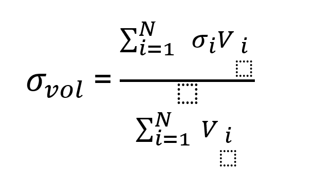
where σ_vol is the volume averaged stress and V_i is the volume of element i. The volume-based weighing approach can also be extended to strain or other elemental quantities.

Volume Averaging with Ansys DPF minimizes numerical errors due to mesh density variations, and localized stress singularities. Volume averaging ensures that highly refined elements do not artificially bias the stress/strain data, making it useful for:

Material Characterization: Comparing simulation zones against macroscopic with experimental results such as creep vs time curves or tensile stress vs strain curves, stress relaxation vs time curves, without localized mesh spikes.
Durability & Fatigue: To extract representative volume-averaged values across a component or “process-zone” rather than relying on individualized, non-physical stress spikes.

3. FEA Model and Loading Setup for Volume Averaging with Ansys DPF

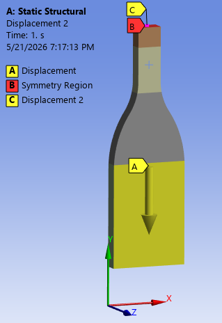
A standard Aluminum 6061 (Al 6061) tensile coupon specimen was selected to perform the volume average calculations. A half-model was utilized to ensure deformation symmetry. The modeling details are presented in Appendix A.

Fig. 1 – Boundary Conditions

Boundary Conditions:

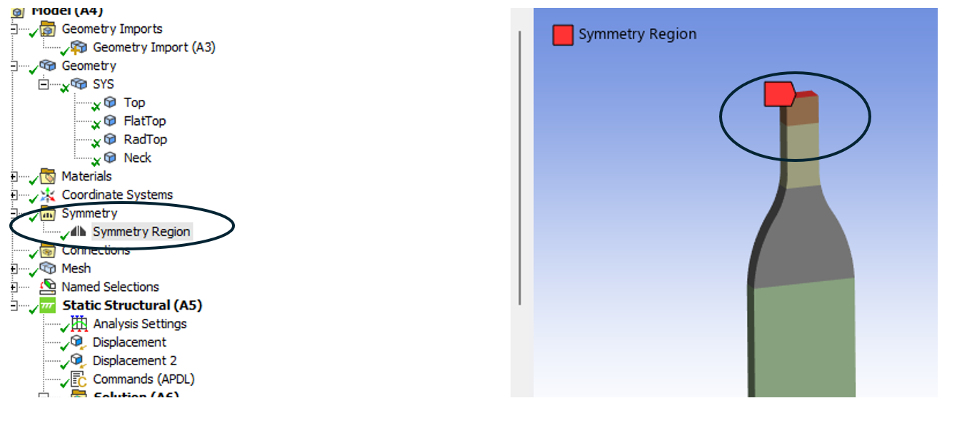
Symmetry: Symmetry constraints are enforced at half plane as shown in Fig. 1. (plane B)
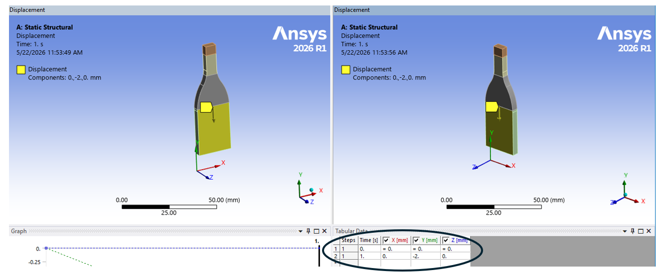
Clamp Region: A uniform axial displacement of 2 mm is applied in the Y-direction (axial loading). To simulate the gripping at the ends, displacement along the other two orthogonal directions (X and Z) are fixed on the clamp faces.
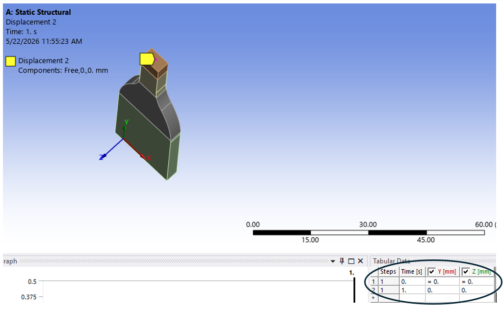
Center of Symmetry Constraint: The center of the symmetry plane was fixed in the X and Z directions to prevent rigid body translation and eliminate unconstrained out-of-plane movements.

Material Properties and Constitutive Modeling

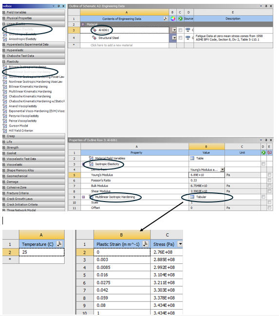
Elasticity: The elastic response of the Al 6061 alloy is modeled using standard isotropic linear elasticity with Young’s Modulus E = 68.9 GPa and Poisson’s Ratio υ =33.
Plasticity: To capture material plasticity of the Al 6061 alloy, a Multilinear Isotropic Hardening model was utilized. Plastic yielding is governed by the standard von Mises criterion, with a uniformly expanding yield surface. The post-yield flow curve is defined using true stress versus equivalent plastic strain data points.

Mesh Sizing and Regional Subdivisions

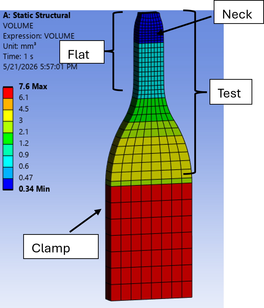
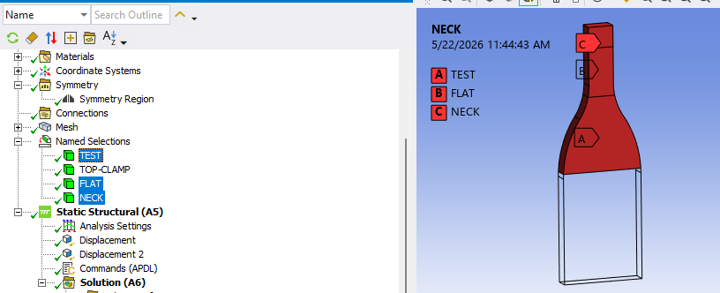
To test the effect of mesh dimensions on extracted elemental quantities, the test region of the coupon was subdivided into three distinct evaluation zones:

Neck Region: The central zone where localized plastic deformation and necking are expected to occur. This zone is meshed with a highly refined, uniform element size of 0.5 mm.
Flat Test Region: This zone encompasses the refined neck region plus the adjacent flat parallel length of the coupon. The elements transitioning into this region have a mesh size of 1.0 mm.
Entire Test Region: This zone encompasses the neck, the flat region, and the transitioning radii leading to the grip sections. The mesh size in this region is approximately 2.0 mm.

Clamp/Grip Region: The outermost region where uniform displacement is applied. A coarse mesh size of 4.0 mm is used in this region. Data from this region is entirely ignored during post-processing extraction due to grip and displacement boundary conditions.

Fig. 2 – Mesh Sizing and Regional Subdivisions

4. Results & Discussions

4.1 Equivalent Plastic Strain Accumulation Over Time (Steps)

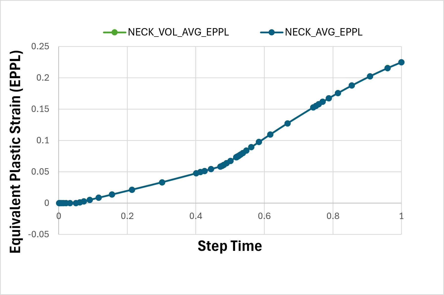
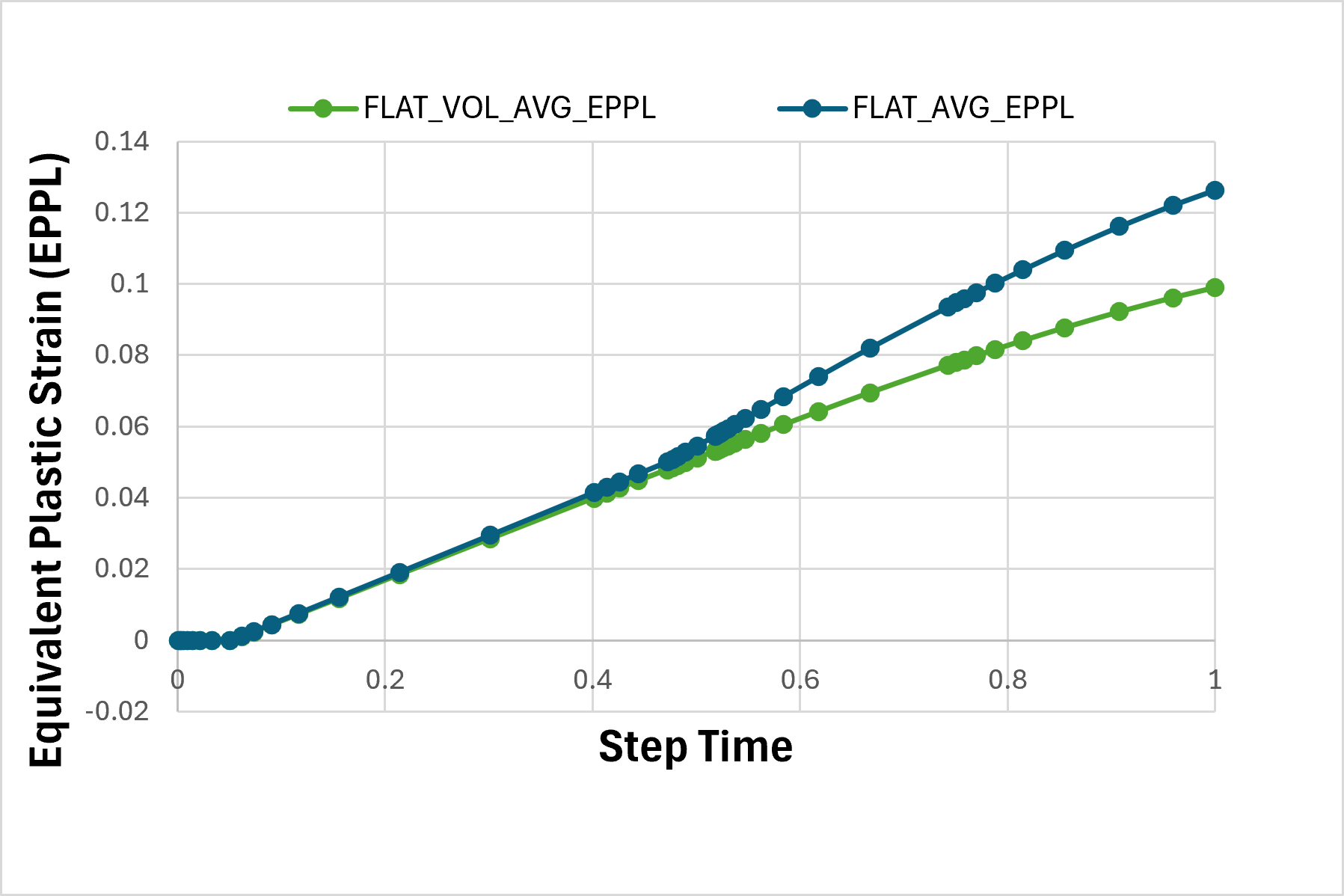
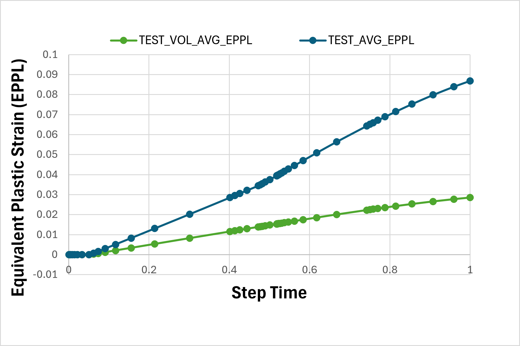
To evaluate the impact of mesh bias over time, equivalent plastic strain accumulation was tracked across all simulation steps for the Neck, Flat, and Test regions and are plotted in Figs. 3a, 3b and 3c:

Neck Region: The volume-averaged and non-weighted arithmetic curves correlate perfectly throughout the entire time history. Because the local mesh is highly uniform, no geometric bias is introduced.
Flat & Test Regions: The two averaging methods severely diverge over time. Because the non-weighted average treats every element equally, the regions of highly refined elements in the neck artificially amplifies the region’s calculated strain.
Volume Averaging: Volume Averaging with Ansys DPF eliminates this artifact by weighing each element’s strain against its actual physical volume. By scaling the high neck strains by their tiny local volumes, it accurately reflects the physical reality that only a small fraction of the total material volume has undergone severe plastic deformation.

Fig. 3a – Equivalent Plastic Strain vs Time (Neck Region)

Fig. 3b – Equivalent Plastic Strain vs Time (Flat Region)

Fig. 3c – Equivalent Plastic Strain vs Time (Test Region)

4.2 Equivalent Stress vs. Equivalent Plastic Strain

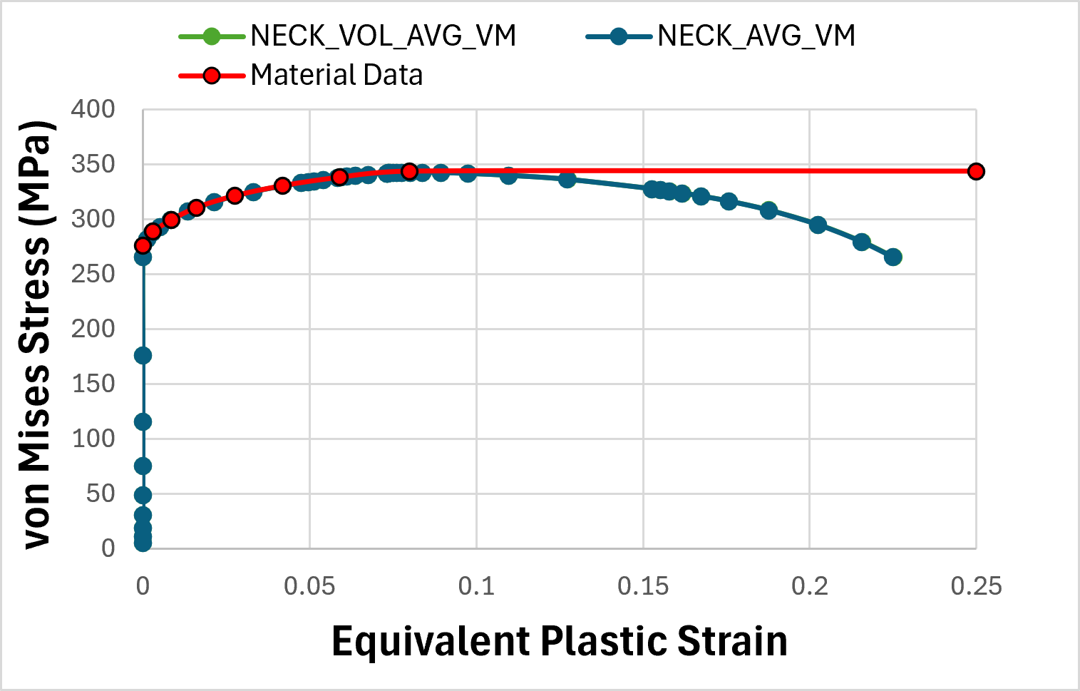
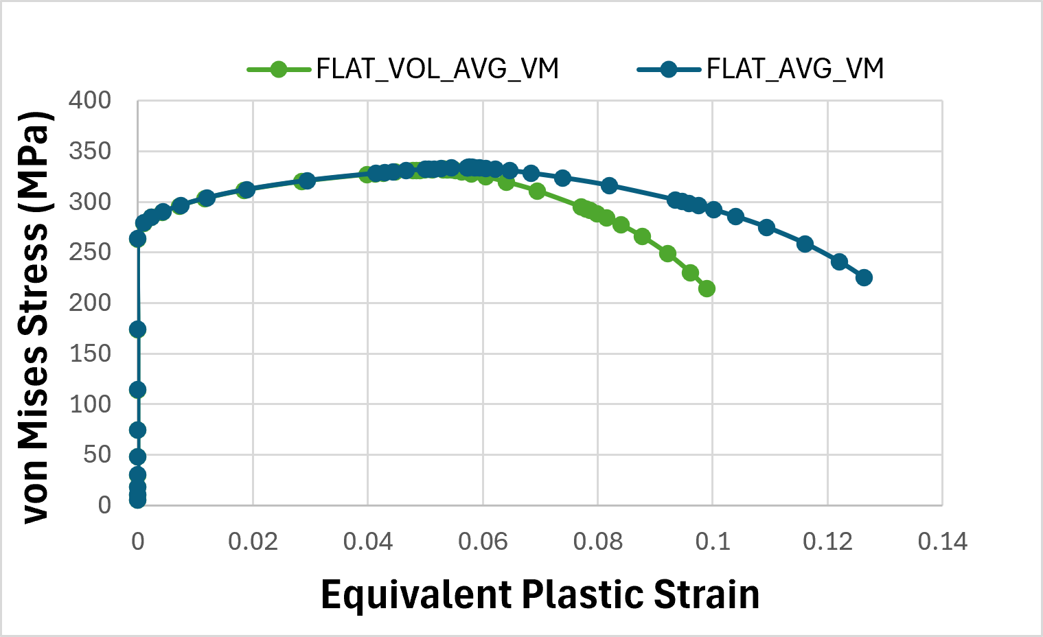
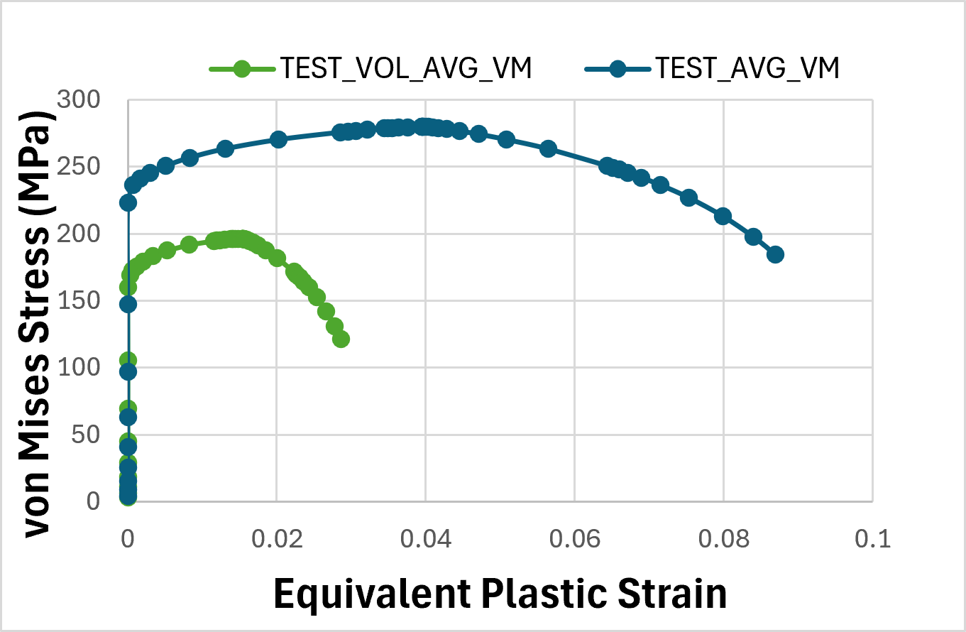
To evaluate the impact of mesh bias on equivalent stress vs equivalent plastic strain, results are plotted for the Neck, Flat, and Test regions shown in Figs. 4a, 4b and 4c:

Neck Region: The volume-averaged and non-weighted arithmetic curves correlate perfectly due to uniform mesh in this region and compare well with material data until necking. After the on-set of necking, partial elastic unloading is noted in the regions adjacent to neck resulting in drop in stress in these regions.

Flat & Test Regions: The non-weighted average exhibits an artificially stiffer behavior and reaches a higher maximum stress (Fig. 4c). Because the highest stresses are localized within the small, highly refined neck elements, giving them equal weight increases the entire regional stress state. The non-weighted curves show higher plastic strain accumulation over time as explained in previous section and this artificially stretches the curve along the X-axis (Fig. 4b and 4c).

Volume Averaging: Volume averaging removes this geometric artifact by scaling the extreme local neck behaviors and the resulting volume-averaged curves undergo early structural softening.

Fig. 4a – Equivalent Stress vs Equivalent Plastic Strain vs Time (Neck Region)

Fig. 4b – Equivalent Stress vs Equivalent Plastic Strain vs Time (Flat Region)

Fig. 4c – Equivalent Stress vs Equivalent Plastic Strain vs Time (Test Region)

5. Volume Averaging with Ansys DPF: In Conclusion

This study shows that non-weighted arithmetic averaging can distort regional FEA results in non-uniform meshes, artificially increasing stiffness, stress, and plastic strain. Volume averaging removes this mesh-density bias and provides more accurate stress–strain behavior, making it essential for reliable material validation and regional post-processing.

This model is intended solely to demonstrate the effects of non-uniform mesh density on simple averaging and weighted averaging, not to predict damage or fracture, which would require carefully chosen ductile damage models.

Improve the Reliability of Your FEA Post-Processing

Mesh refinement should improve solution accuracy—not distort the regional data used to evaluate material behavior, durability, or structural performance. Ansys DPF enables engineers to automate volume-weighted result extraction directly from Ansys result files, reducing mesh-density bias and supporting more reliable stress and strain comparisons.

SimuTech Group can help you develop customized Ansys post-processing workflows, automate repetitive result extraction, and apply advanced FEA techniques to your engineering models.

Talk with an Ansys expert about your FEA post-processing needs.

Gayathri Venkataramani, M.Eng. Structural Engineering
Staff Engineer – Structures, SimuTech Group

Gayathri Venkataramani is a Staff Engineer in Structures at SimuTech Group. She specializes in finite element analysis, structural simulation, and advanced post-processing using Ansys software. Her work includes developing practical methods for extracting reliable engineering data, reducing mesh-dependent bias, and automating simulation workflows with tools such as the Ansys Data Processing Framework.

Geometry:

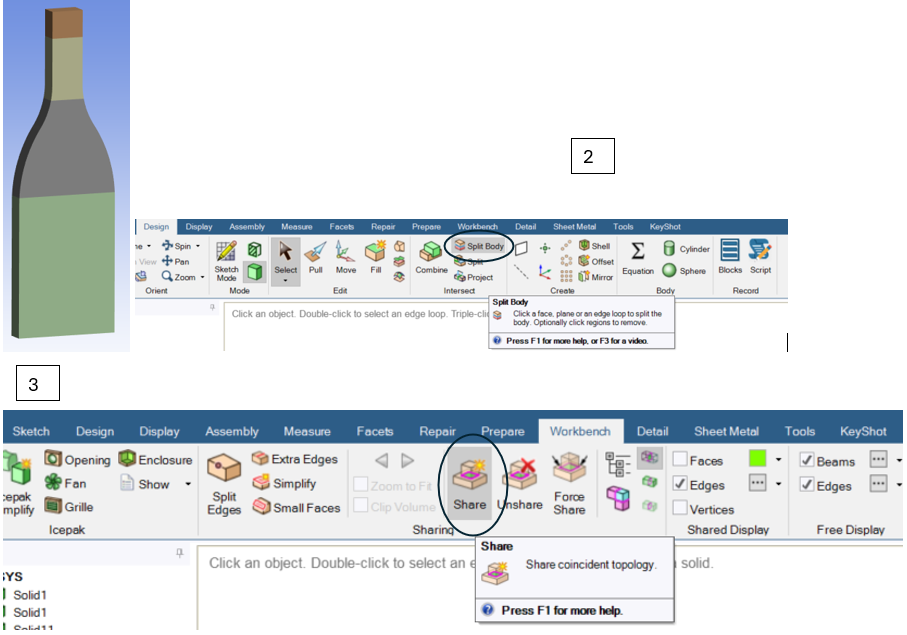
1 – Half – Geometry was created in space claim.
2 – Split bodies in space claim to define meshing zone for various regions
3 – Share topology (under Workbench Menu) to ensure mesh is matched across interfaces

Material Data:

Create New Material – Al 6061 with following Properties. Isotropic Elasticity and Plasticity à Multilinear Isotropic Hardening.

FEA Model:

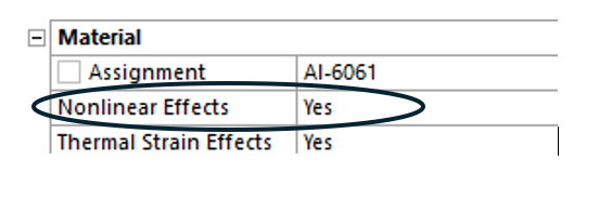
1. Assign Al-6061 to all the solid bodies under Geometry. Make sure Nonlinear Effects are set to Yes

2. Insert Symmetry Region as shown below

3. Create Named Selection as shown below. These names will be used to extract specific element sets for post processing.

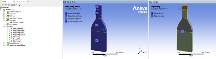
4. Meshing is controlled as desired by using Body Sizing and Edge Sizing options

5. Apply boundary conditions – Displacement of -2mm on both faces (to simulate clamp). Displacement on center node of symmetry to prevent out of plane movements.

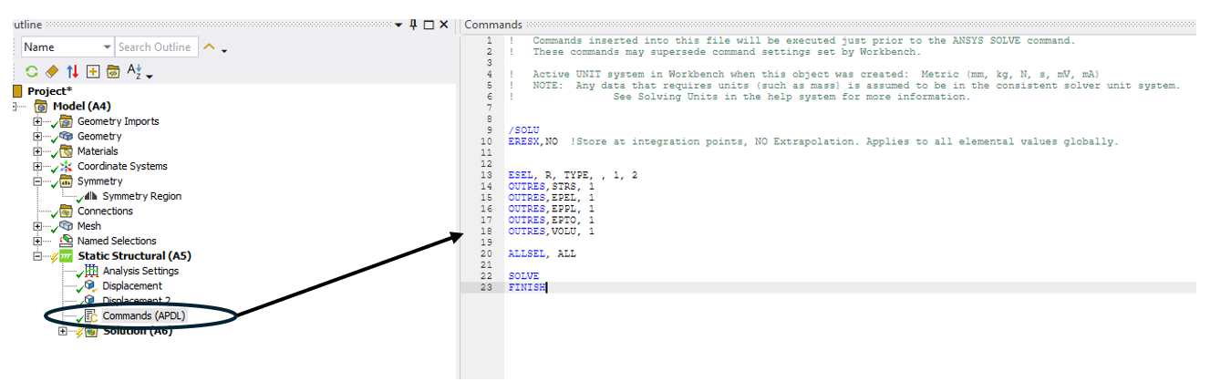
6. Following command snippet is used under Static Structural to store element values at integration points at every converged time step.

7. Below analysis settings were chosen. Large deflection to be ON. Time stepping to be smaller to help in convergence especially beyond the onset of necking.

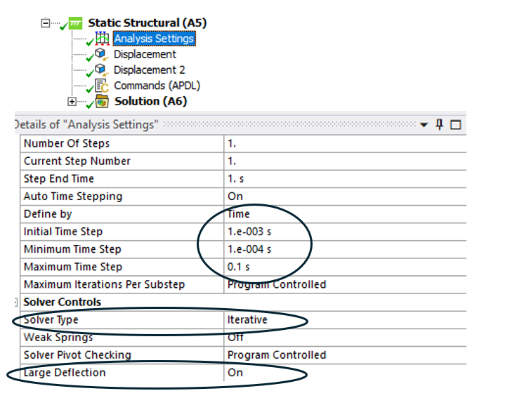
The model is ready to be solved for further post processing!

Ansys DPF Extraction Framework

In our volume averaging with Ansys DPF example, Python with the Ansys Data Processing Framework (DPF) was utilized. The automation script follows the workflow as shown below:

Geometry Scoping: Predefined Named Selections (NECK, FLAT, and TEST) are mapped to their corresponding elemental mesh scopings.
DPF Operators: Elemental stress, equivalent plastic strain, and elemental volume operators are created and configured for all simulation time steps.
Calculation: Elemental stress tensors and strain data are evaluated through DPF and processed using NumPy to compute scalar von Mises stress and equivalent plastic strain values.
Weighted Integration: For each Named Selection and time step, both volume-weighted and non-weighted arithmetic averages are computed for comparison.

The script is executed in a Python environment (Jupyter Notebook or equivalent), where the user defines the input path to the Ansys result file (.rst) (.dat) file and the output directory for storing processed results.

Post-Processing Script

import ansys.dpf.core as dpf
import numpy as np
import csv

#Load Model
model = dpf.Model(r”C:\Path\file.rst”)
mesh = model.metadata.meshed_region

#Named Selections
print(mesh.available_named_selections)

#Scoping Named Selections
neck_scoping = mesh.named_selection(“NECK”)
flat_scoping = mesh.named_selection(“FLAT”)
test_scoping = mesh.named_selection(“TEST”)

scopings = {
“NECK”: neck_scoping,
“FLAT”: flat_scoping,
“TEST”: test_scoping
}
#Time Scoping
time_scoping = model.metadata.time_freq_support.time_frequencies.scoping

# Stress Operator
stress_op = model.results.stress()
stress_op.inputs.requested_location.connect(“Elemental”)
stress_op.inputs.time_scoping.connect(time_scoping)

# Volume Operator
vol_op = model.results.elemental_volume()
vol_op.inputs.time_scoping.connect(time_scoping)

# Plastic Strain Operator
eppl_op = model.results.plastic_strain()
eppl_op.inputs.requested_location.connect(“Elemental”)
eppl_op.inputs.time_scoping.connect(time_scoping)

# Evaluate For Time Looping
stress_fc = stress_op.eval()
set_ids = stress_fc.get_label_scoping(“time”).ids
times = stress_fc.time_freq_support.time_frequencies.data

print(set_ids)
print(times)

#von Mises Stress Calculation
def von_mises(s):

sxx = s[:, 0]
syy = s[:, 1]
szz = s[:, 2]
sxy = s[:, 3]
syz = s[:, 4]
sxz = s[:, 5]

return np.sqrt(
0.5 * (
(sxx – syy) ** 2 +
(syy – szz) ** 2 +
(szz – sxx) ** 2 +
6 * (sxy ** 2 + syz ** 2 + sxz ** 2)
)
)

#Equivalent Plastic Strain Calculation

def equivalent_plastic_strain(ep):

exx = ep[:, 0]
eyy = ep[:, 1]
ezz = ep[:, 2]
exy = ep[:, 3]
eyz = ep[:, 4]
exz = ep[:, 5]

return np.sqrt(
(2.0 / 3.0) * (
exx ** 2 +
eyy ** 2 +
ezz ** 2 +
0.5 * (
exy ** 2 +
eyz ** 2 +
exz ** 2
)
)
)

#Main Loop For Calculations
results = []
for i, step in enumerate(set_ids):
row = [step, times[i]]
for name, scoping in scopings.items():

stress_op.inputs.mesh_scoping.connect(scoping)
eppl_op.inputs.mesh_scoping.connect(scoping)
vol_op.inputs.mesh_scoping.connect(scoping)

stress_fc = stress_op.outputs.fields_container()
eppl_fc = eppl_op.outputs.fields_container()
vol_fc = vol_op.outputs.fields_container()

stress = stress_fc[i].data
eppl = eppl_fc[i].data
vol = vol_fc[i].data

s22 = stress[:, 1]
e22 = eppl[:, 1]

vm = von_mises(stress)
eqv_eppl = equivalent_plastic_strain(eppl)

#Volume Averaging and Mean Calculations
total_vol = np.sum(vol)

vol_avg_s22 = np.sum(s22 * vol) / total_vol
vol_avg_e22 = np.sum(e22 * vol) / total_vol
vol_avg_vm = np.sum(vm * vol) / total_vol
vol_avg_eqv_eppl = np.sum(eqv_eppl * vol) / total_vol

avg_s22 = np.mean(s22)
avg_e22 = np.mean(e22)
avg_vm = np.mean(vm)
avg_eqv_eppl = np.mean(eqv_eppl)

#Results
row.extend([
vol_avg_s22,
vol_avg_e22,
vol_avg_vm,
vol_avg_eqv_eppl,
avg_s22,
avg_e22,
avg_vm,
avg_eqv_eppl
])

results.append(row)

#Write Output File
output_file = r”C:\Path\Tensile_Results.csv”

header = [“Step”, “Time”]

for name in scopings.keys():
header.extend([
f”{name}_VOL_AVG_S22″,
f”{name}_VOL_AVG_E22″,
f”{name}_VOL_AVG_VM”,
f”{name}_VOL_AVG_EPPL”,
f”{name}_AVG_S22″,
f”{name}_AVG_E22″,
f”{name}_AVG_VM”,
f”{name}_AVG_EPPL”
])

with open(output_file, “w”, newline=””) as f:
writer = csv.writer(f)
writer.writerow(header)
writer.writerows(results)

print(“Saved to:”, output_file)