Oscillatory Mixing Using Ansys Fluent Dynamic Mesh

Challenges of Gentle Mixing in Oscillatory Reservoir Systems

Designing oscillatory reservoir mixing systems for buffers and reagents presents several fluid dynamics challenges that are well suited for Computational Fluid Dynamics (CFD) analysis. Engineers must achieve sufficient mixing uniformity while avoiding excessive shear stress that could damage sensitive biological materials or alter reagent performance. Another challenge is minimizing unwanted flow through inlet and outlet openings during wall oscillation, since pressure fluctuations can induce leakage or backflow. Dead zones, recirculation regions, and stagnant pockets can also reduce mixing effectiveness and create concentration gradients. Additionally, oscillatory motion introduces transient flow behavior that can be difficult to characterize experimentally, especially when geometry, oscillation frequency, and fluid properties interact in complex ways.

Engineering Solutions for Oscillatory Reservoir Mixing Systems

To address these challenges, engineers incorporate oscillating wall motion, carefully tuned displacement amplitudes, and optimized oscillation frequencies to generate controlled recirculation without producing excessive strain. Reservoir geometry may be modified with rounded corners, internal contours, or baffles to eliminate stagnant regions and improve circulation patterns. In many systems, low-Reynolds-number mixing strategies are preferred to maintain gentle agitation while enhancing diffusion-driven transport between the buffer and reagent. Engineers may also evaluate multiple wall motion profiles, including sinusoidal or phase-shifted oscillations, to balance mixing efficiency with pressure stability. These design approaches aim to maximize homogenization while protecting sensitive materials and maintaining predictable transient flow behavior.

Evaluating Oscillatory Mixing Using Ansys Fluent

Ansys Fluent provides a powerful CFD platform for evaluating oscillatory reservoir mixing systems using transient simulations with dynamic mesh capabilities. Dynamic mesh methods allow moving walls to oscillate realistically while continuously deforming the computational domain to capture time-dependent fluid motion. Engineers can use Fluent to analyze velocity fields, vorticity, shear strain, pressure fluctuations, and species concentration transport throughout the oscillation cycle. Parametric studies can then be performed to compare oscillation amplitudes, frequencies, wall motion strategies, and reservoir geometries. CFD visualization also helps identify stagnant regions, excessive strain zones, and unwanted leakage through openings. By combining transient flow physics with dynamic mesh modeling, Ansys Fluent enables engineers to optimize gentle mixing performance before physical prototyping or experimental validation.

Simulation Geometry

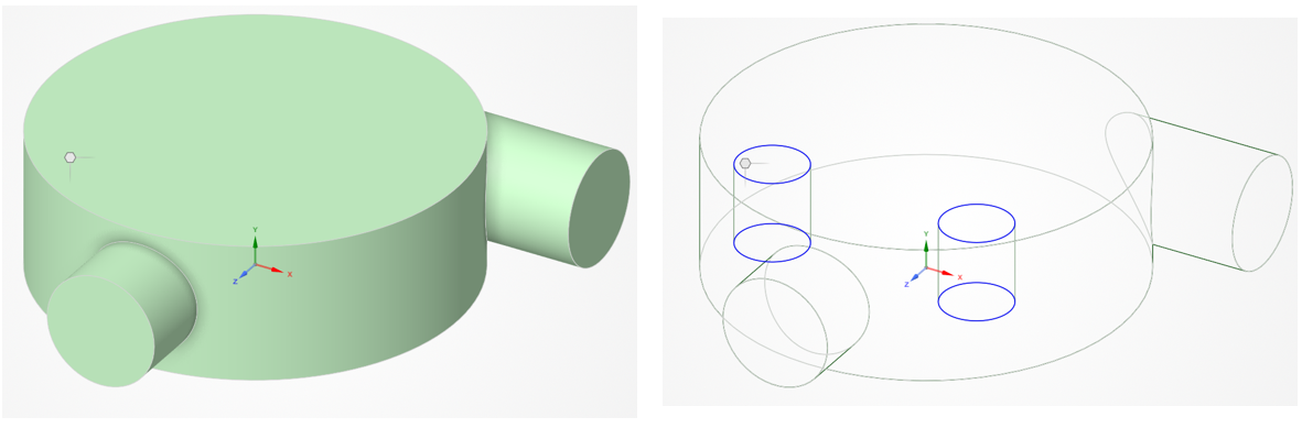
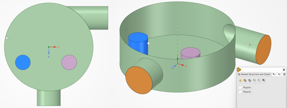
The geometry for this example simulation is a shallow cylinder with two ports. The ports are orientated 90 degrees with respect to each other.  One is directed toward the axis of the cylinder and the other is directed offset from the axis.  Two cylinders are placed inside the cylinder for the purpose of representing the initial deposition of a reagent fluid.  These cylinders will be used to initialize the reagents at the beginning of the transient simulation.  Named selections are recommended to label the ports. This geometry will be meshed with polyhedral mesh elements.  Extruded mesh zones will be grown outward from these labeled surfaces.

Simulation Mesh

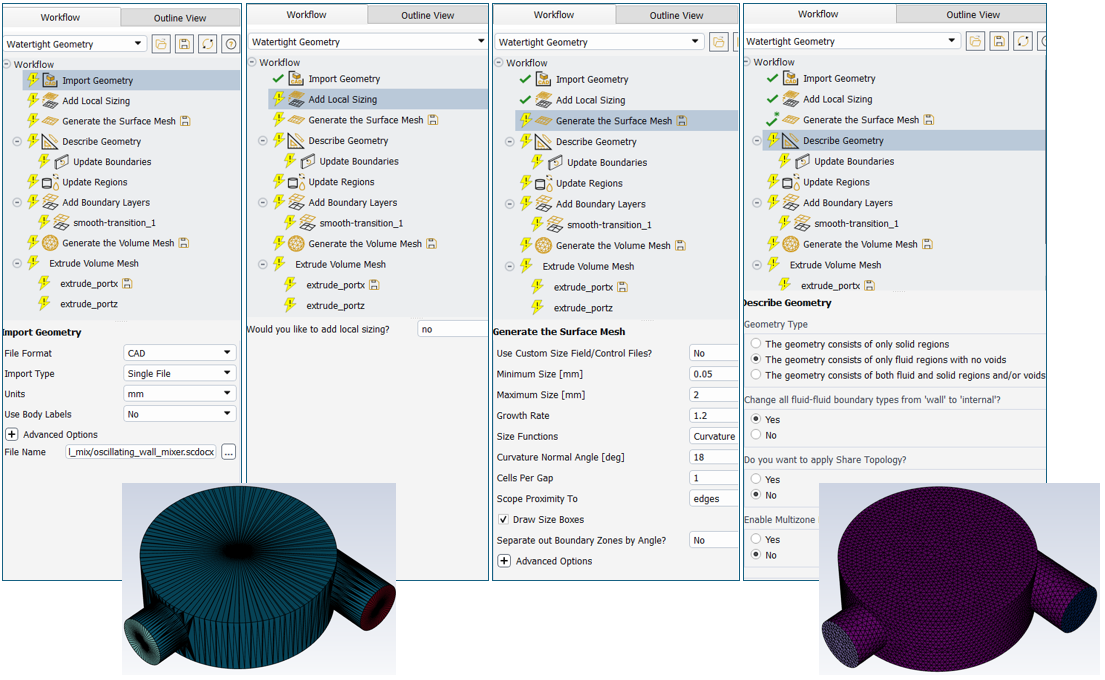
Fluent Mesh Mode is used to generate the volume mesh for oscillatory mixing using Ansys Fluent. The Watertight workflow is used. Geometry is imported using units of [mm], no Local Sizings are used, and the global minimum and maximum mesh sizes are 0.05 [mm] and 2.0 [mm], respectively. The geometry is described as fluids-only.

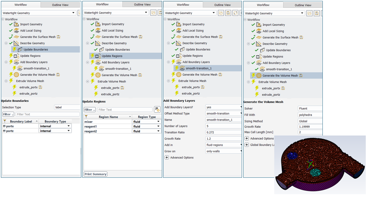
The named selections are set to the “internal” boundary type. The regions are all fluid. Five smooth-transition boundary layers are grown from the walls of the fluid regions. Polyhedral mesh elements fill the regions with a maximum size of 2.0 [mm].

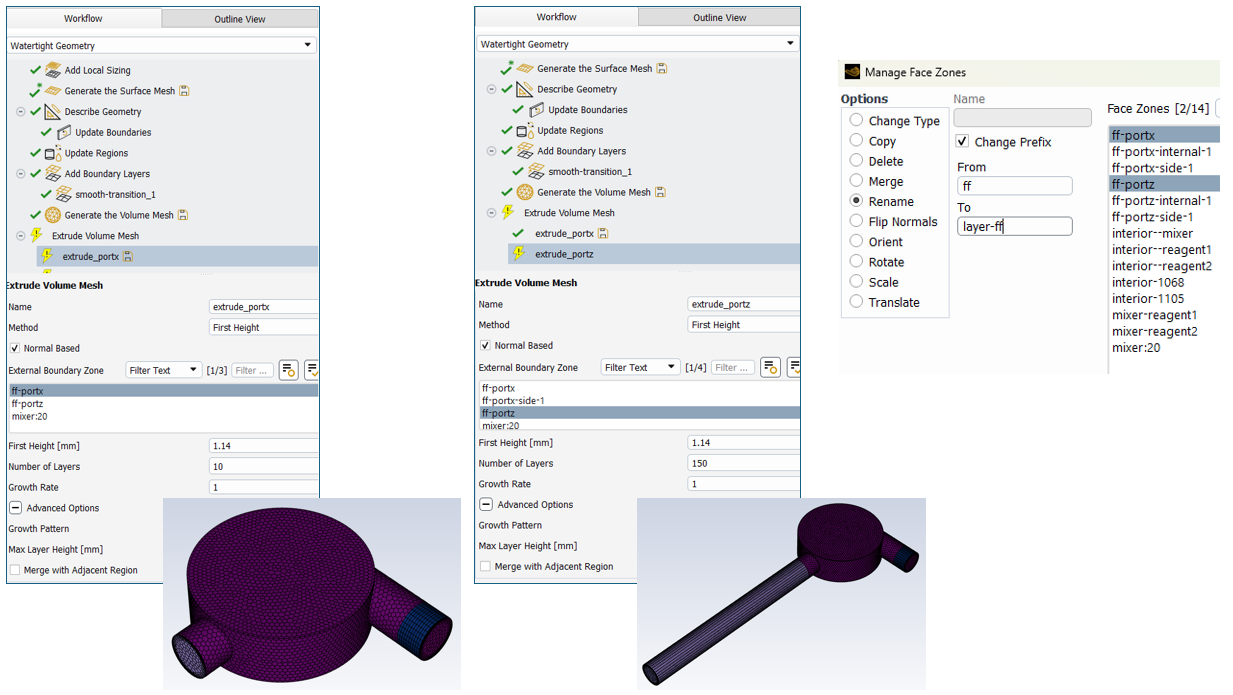
Two extrusions are generated. Extrusion meshes are needed for the Fluent dynamic mesh to work properly. Both extrusions use a growth rate of 1.0 and a first height of 1.14 [mm], and neither is merged with the adjacent region. The extrusion from ff-portx is short, with 10 layers, because its layering surface will initially move away from the reservoir cylinder. The extrusion from ff-portz is tall, with 150 layers, because its layering surface will initially move toward the reservoir cylinder. The volume of this extrusion is set to be at least 45% of the cylindrical reservoir. Renaming the top surface of each extrusion is recommended so these zones can be located readily in Solver Mode.

Simulation Setup

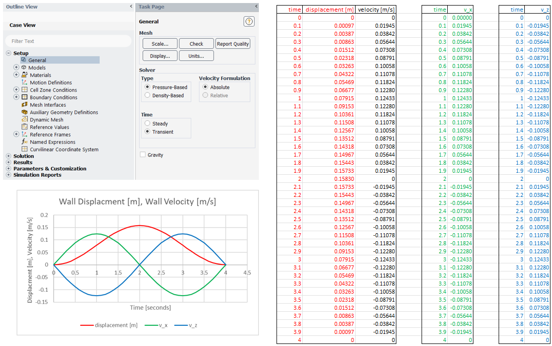
The simulation for oscillatory mixing using Ansys Fluent is transient. The top face zones of the extrusion zones move sinusoidally with a maximum displacement of 0.1583 [m] and a cycle period of 4 seconds. The motion velocity is obtained by taking the time derivative of the displacement. Transient table profiles can then be generated from the velocity. The profile for portx starts with a positive velocity in the X-coordinate direction, while the profile for portz starts with a negative velocity in the Z-coordinate direction. The profiles should be saved as text files and read into the Fluent solver with the periodic flag activated. The header for the portx profile is “profile_v_x 2 41 1,” and the header for the portz profile is “profile_v_z 2 41 1.” The number 2 indicates the number of columns in the profile, and 41 indicates the number of rows.

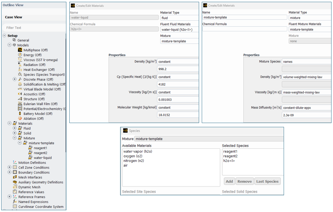
The simulation is single-phase and includes multiple species. The mixture contains water and two reagents, with each species assigned the properties of water. The mixture uses volume-weighted density, mass-weighted viscosity, and a constant mass diffusivity.

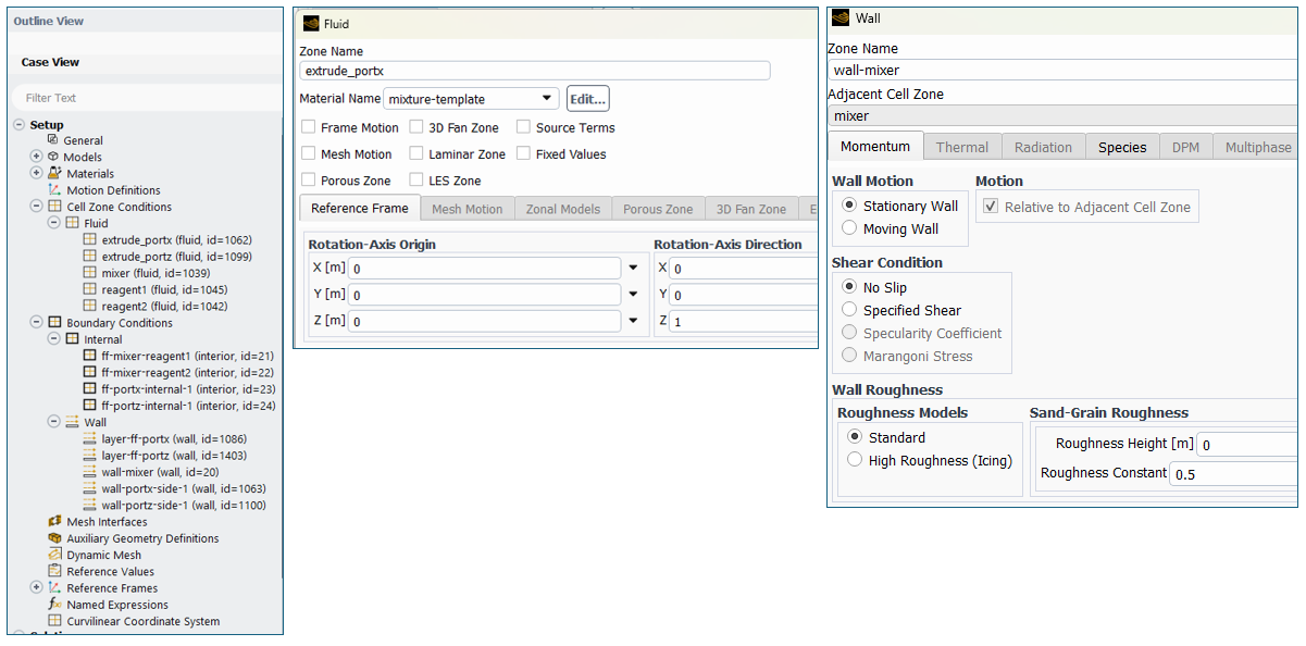
All fluid cell zones use the mixture template as the material. All walls are assigned a no-slip shear condition.

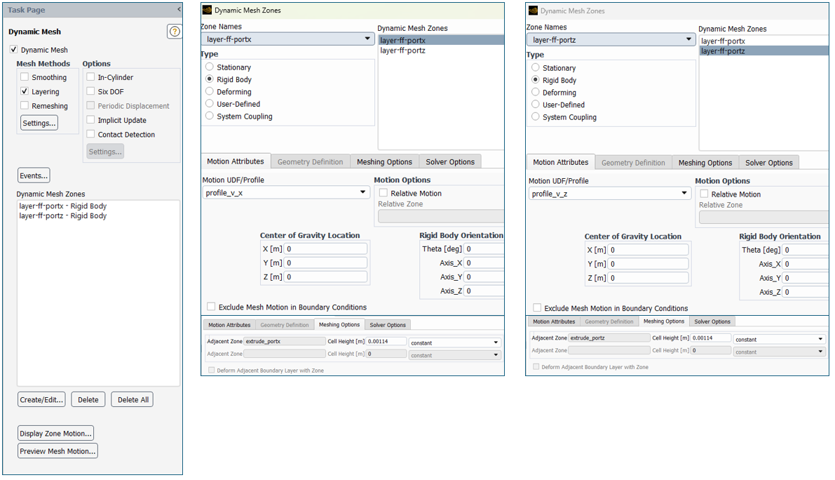
The dynamic mesh model is activated, and all methods and options are deactivated except for Layering. A dynamic mesh zone is created for layer-ff-portx using the profile_v_x motion profile, and another dynamic mesh zone is created for layer-ff-portz using the profile_v_z motion profile. The cell height is set to 0.00114 [m] in the Meshing Options tab.

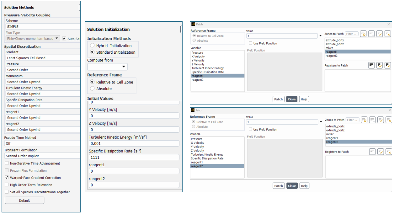
The domain should be initialized with a zero mass fraction for each reagent. The mass fraction of reagent1 should then be patched to 1 in its cell zone, and the mass fraction of reagent2 should be patched to 1 in its cell zone. A second-order implicit transient formulation is recommended.

Fluent Named Expressions can be used to generate reports and monitors that assess mixing performance over time. One recommended metric is the fractional volume unmixed. The expressions below calculate the fractional volume unmixed for a target mixing level of 95%.

volavemfmata: max(1e-16,VolumeAve(MassFraction(species = ‘reagent1’),[“extrude_portx”,”extrude_portz”,”mixer”,”reagent1″,”reagent2″]))

volavemfmatb: max(1e-16,VolumeAve(MassFraction(species = ‘reagent2’),[“extrude_portx”,”extrude_portz”,”mixer”,”reagent1″,”reagent2″]))

upperlimit95a: 1.025*volavemfmata

upperlimit95b: 1.025*volavemfmatb

lowerlimit95a: 0.975*volavemfmata

lowerlimit95b: 0.975*volavemfmatb

aboveflag95a: IF(MassFraction(species = ‘reagent1’) > upperlimit95a,1,0)

aboveflag95b: IF(MassFraction(species = ‘reagent2’) > upperlimit95b,1,0)

belowflag95a: IF(MassFraction(species = ‘reagent1’) < lowerlimit95a,1,0)

belowflag95b: IF(MassFraction(species = ‘reagent2’) < lowerlimit95b,1,0)

flags95a: aboveflag95a+belowflag95a

flags95b: aboveflag95b+belowflag95b

myfractionalvolume95:

Sum(CellVolume*IF(flags95a>0,1.0,0.0),[“extrude_portx”,”extrude_portz”,”mixer”,”reagent1″,”reagent2″])/Volume([“extrude_portx”,”extrude_portz”,”mixer”,”reagent1″,”reagent2″])

myfractionalvolume95: Sum(CellVolume*IF(flags95b>0,1.0,0.0),[“extrude_portx”,”extrude_portz”,”mixer”,”reagent1″,”reagent2″])/Volume([“extrude_portx”,”extrude_portz”,”mixer”,”reagent1″,”reagent2″])

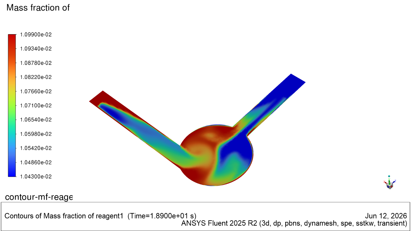
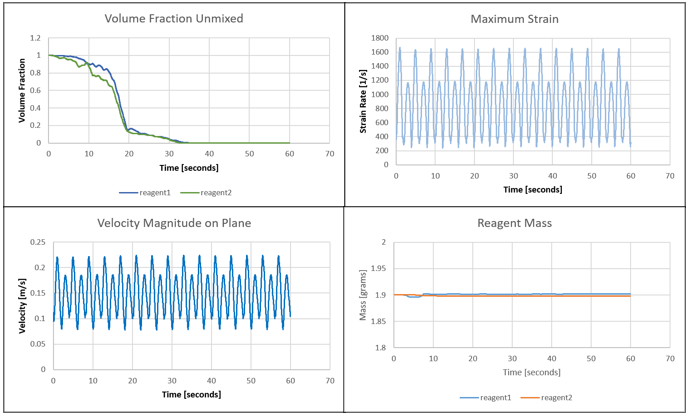
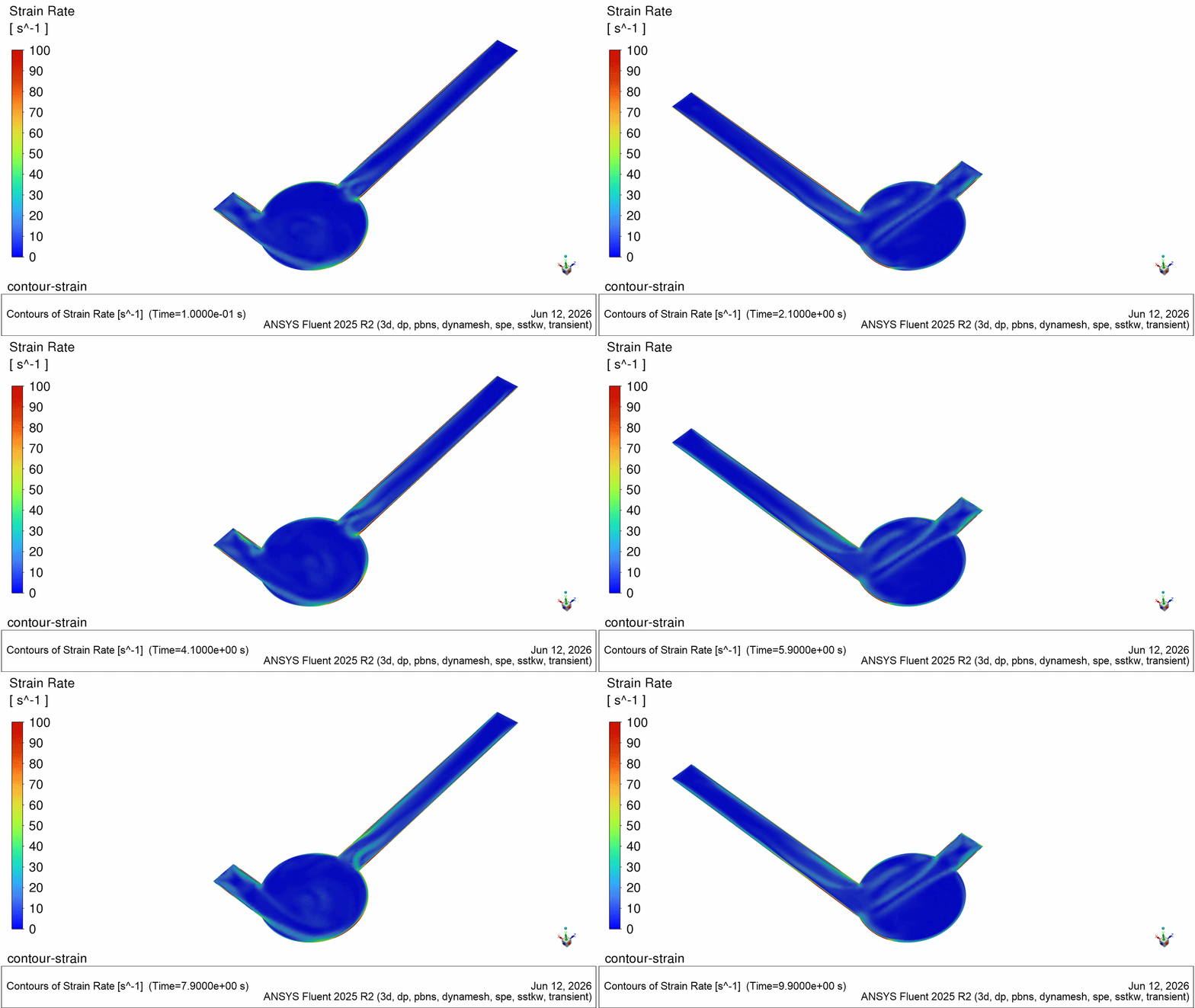
Report Definitions should be generated to monitor the mixing. Report definitions such as fractional volume unmixed, strain rate, velocity magnitude, and reagent mass should be generated for monitors. The volume fraction unmixed monitor plot below indicates different mixing rates for the reagents because of their initial location, and it indicates mixing threshold is reached within 40 seconds.  The maximum strain and maximum velocity monitors indicate the highest strain and velocity in the center plane time, and they indicate that the flow is different based on port flow directionality.  The reagent mass monitor confirms that mass is conserved in the domain for each reagent species.

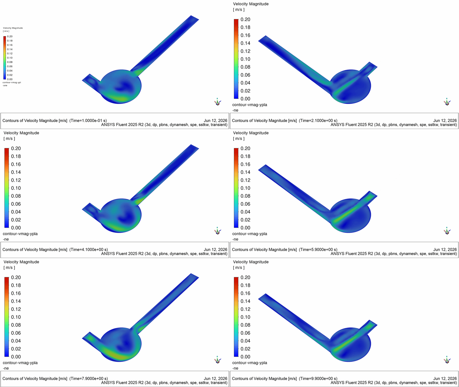
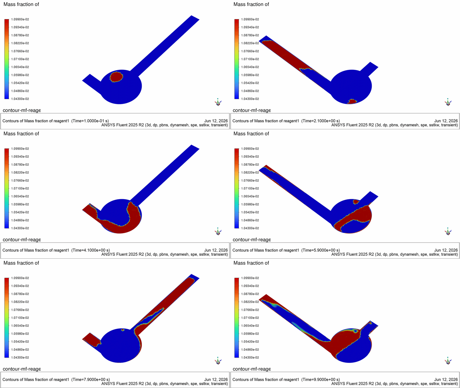
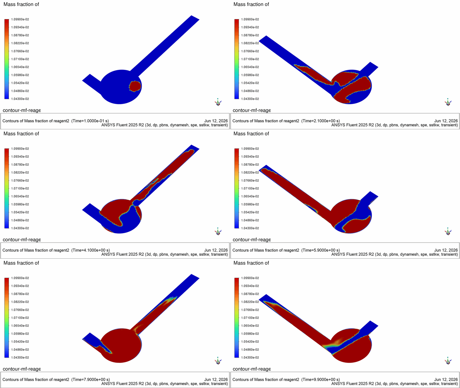
Animated contour plots on the center plane can show the velocity, mass fractions, and the strain rate as the solution progresses.

Video of Oscillatory Mixing Using Ansys Fluent Simulation Setup

The following video walks through the simulation setup from the geometry to meshing to flow solver.

Optimize Oscillatory Mixing with Ansys Fluent

Oscillatory mixing systems must achieve uniform reagent distribution without creating excessive strain, stagnant regions, or unwanted flow through system openings. SimuTech Group’s fluids experts can help you use Ansys Fluent dynamic mesh, species transport, and transient CFD simulations to evaluate mixing time, wall motion, strain rate, and reservoir performance before physical testing.

Talk to a CFD Expert