Rod Pump Simulation Using Ansys Fluent Dynamic Mesh

Challenges of Designing Rod Pumps

Rod pump performance is strongly influenced by internal fluid dynamics, making several design challenges well suited for Computational Fluid Dynamics simulation and analysis. One major issue is multiphase flow behavior involving oil, gas, and produced water moving through the pump barrel and valve regions. Gas interference can reduce pump flow rate and create unstable pressure fluctuations that lower volumetric efficiency. Engineers also face problems related to turbulence, flow separation, cavitation, and recirculation zones near the standing and traveling valves. Transient flow effects generated by the reciprocating plunger motion can produce localized pressure spikes and unsteady velocity fields that negatively impact hydraulic efficiency and overall pump performance.

Engineering Solutions for Rod Pump Performance

Many of these hydraulic challenges can be addressed through engineering solutions focused on improving internal flow behavior. Optimized valve geometries can reduce pressure losses, improve sealing performance, and minimize turbulent recirculation during valve opening and closing cycles. Modified plunger clearances and barrel designs can improve flow uniformity while reducing leakage and dead zones inside the pump chamber. Gas handling performance can also be improved through redesigned intake geometries and flow paths that promote better gas-liquid separation before fluid enters the pump. Engineers frequently evaluate alternative flow channel shapes and valve lift configurations to reduce cavitation risk, stabilize transient pressure behavior, and improve volumetric efficiency across varying operating conditions.

Using Ansys Fluent to Evaluate Design Solutions

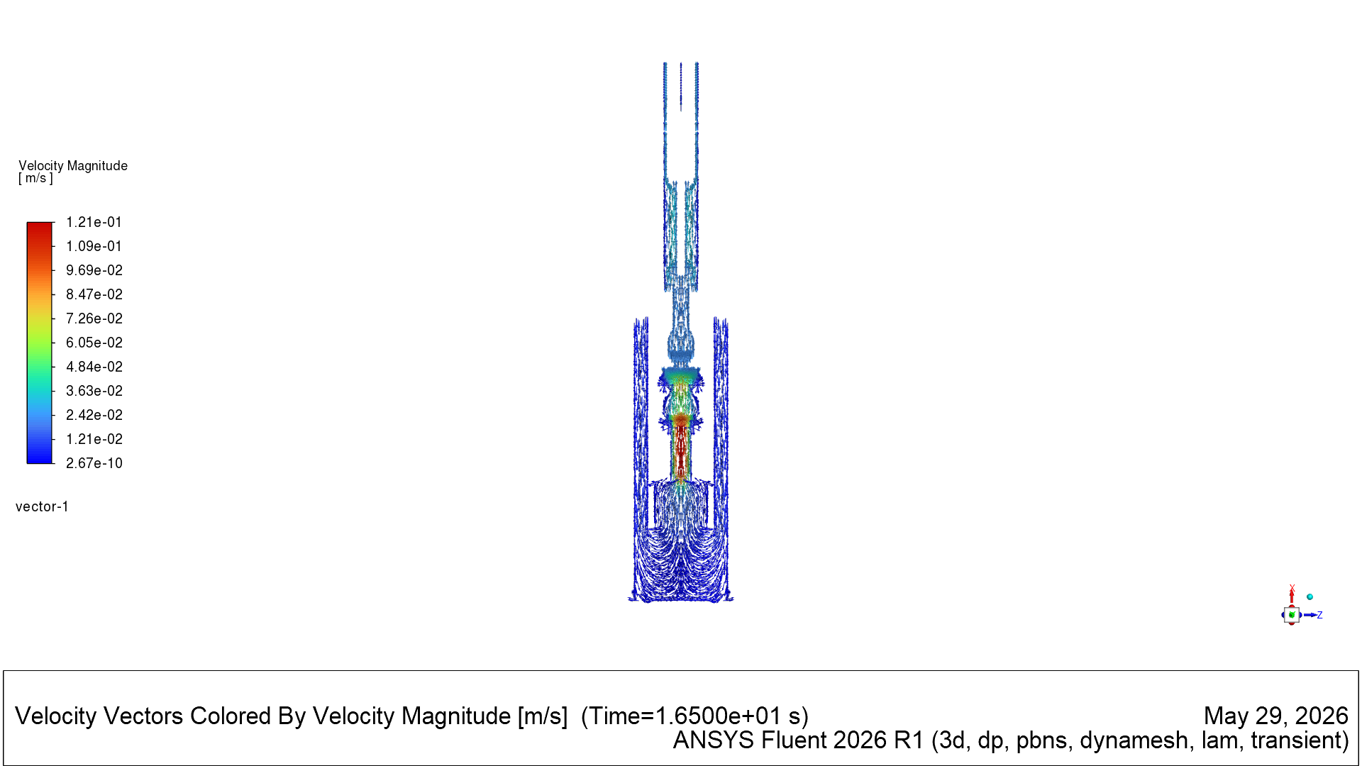
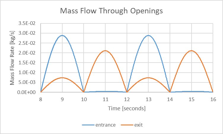
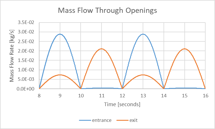
Ansys Fluent with dynamic mesh technology enables engineers to analyze this transient hydraulic phenomena in detail. Dynamic mesh methods allow the computational domain to deform continuously as the plunger and valves reciprocate, accurately representing the physical pump motion during operation. CFD simulations can predict transient pressure fields, velocity distributions, turbulence intensity, cavitation regions, and multiphase flow patterns throughout the pumping cycle. The example graphic below displays velocity vectors on a section plane through a pump, and the example chart below displays pump flow rates through openings. Engineers can visualize recirculation zones, identify inefficient flow regions, and compare alternative valve or intake designs before manufacturing prototypes. Fluent’s multiphase and turbulence models can also provide valuable insight into gas interference and flow instability, helping manufacturers optimize rod pump hydraulic performance and improve operational efficiency.

Analysis Objective

The objective of this simulation is to understand the transient flow rate of oil through a rod pump.  The simulation approach includes dynamic mesh capability within Ansys Fluent to move the plunger up and down in a sinusoidal fashion.  A two dimensional simulation is possible if all the non-planar surfaces are surfaces of revolution.  In this example, a one-quarter model is used to lower mesh count instead.  The geometry should be set such that both the lower and upper plunger positions are feasible for meshing.  The geometry should also be decomposed to include valve regions.

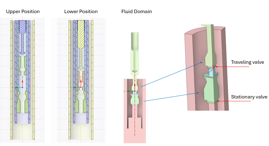
Rod Pump Simulation Mesh

The simulation domain is meshed for flow simulation using Fluent Meshing Mode. The watertight workflow is employed to complete all the necessary steps.  This workflow requires a watertight geometry from the geometry preprocessor.  The workflow contains task steps that include local and global surface mesh sizes, region classification, boundary classification, boundary specification, unstructured volume meshing, and extrusion meshing.

Dynamic mesh with Fluent imposes some requirements on the mesh.  The dynamic mesh will use layering to generate extrusion mesh elements next to a surface that is perpendicular to the motion direction.  One requirement is that the mesh next to the moving face also be a prism shape and not polyhedral.  If a polyhedral mesh element is next to a layering surface, the dynamic mesh will simply stretch the cells next to the surface or compress them, depending on motion direction. As a consequence, the mesh contains several cell zones that are generated with extrusion while others can be unstructured polyhedral.

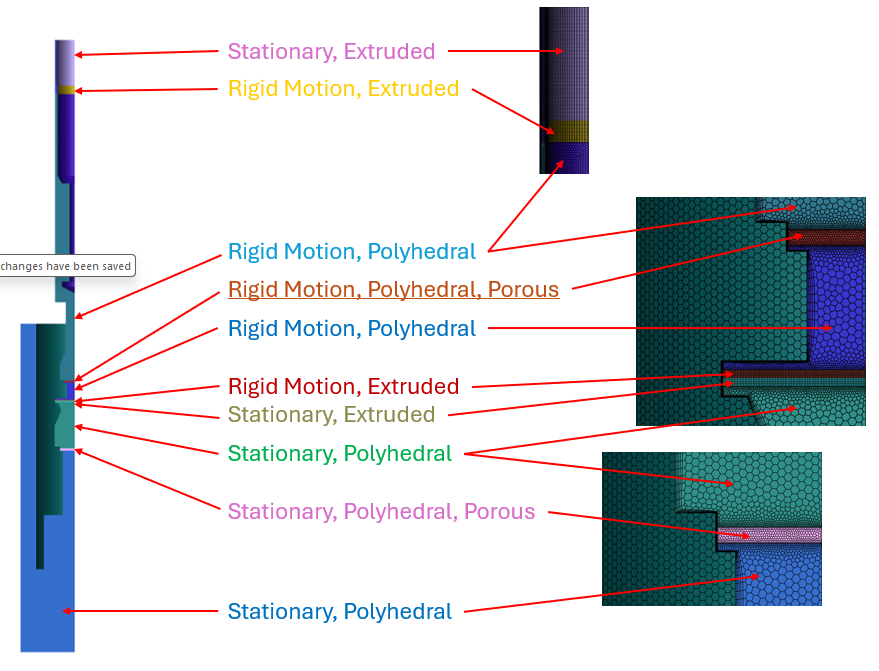
Extrusion meshes are generated in Fluent Mesh Mode after the Generate Volume Mesh task.  In the case of the rod pump simulation, several extrusion meshes are generated, one per sub-task.  Typically conformal meshes are generated in Fluent Mesh mode; however, one non-conformal mesh interface will be generated to accommodate the extrusion mesh requirement.  The starting point for the mesh is the geometry which can be purely polyhedral (or poly-hexcore).  Below are typical workflow tasks for mesh generation up through generating the polyhedral volume mesh.

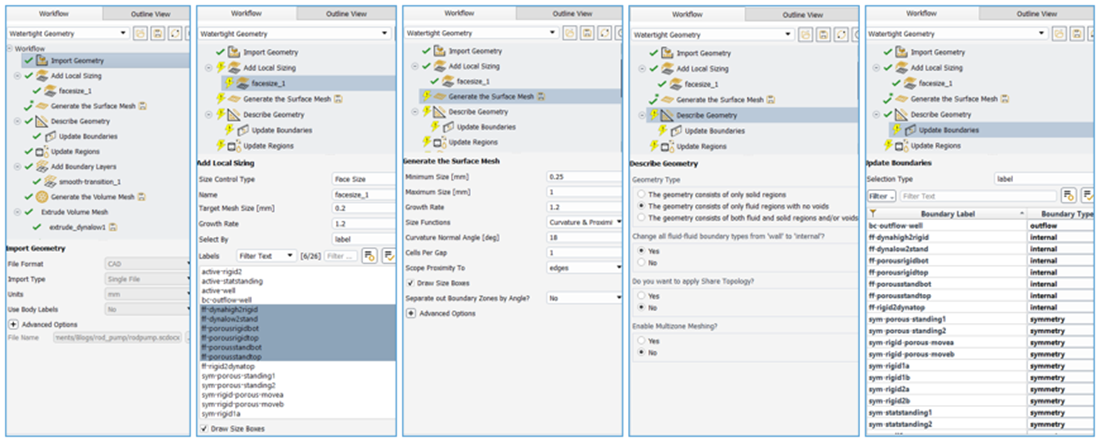
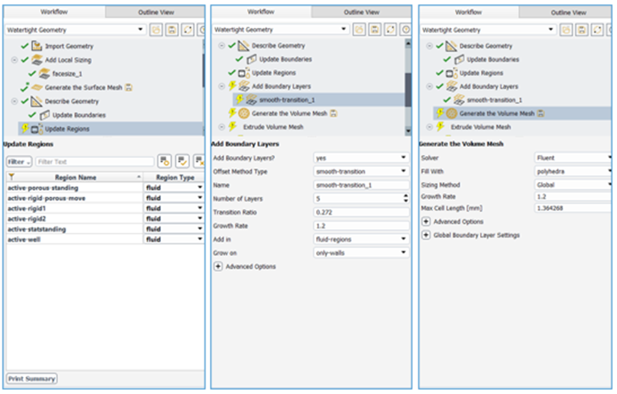
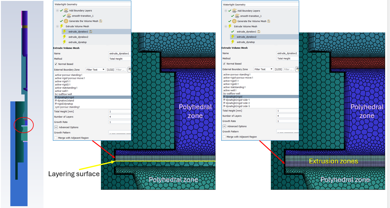
After the watertight workflow is followed to generate the polyhedral mesh, extrusion meshing can begin.  It is best to deactivate the “Merge with Adjacent Region” option in each extrusion sub-task.

Extrusion “extrude_dynalow1” below creates an extrusion near the stationary valve, and the “extrude_dynalow2” creates a second one beyond the first.  The internal face between these extrusion will be a surface for layering in the dynamic mesh.  The final surface of the second extrusion should reach down to a face of the polyhedral mesh, and these two surfaces should be specified as interface-type surfaces.  A mesh interface will be needed in Fluent to permit flow.

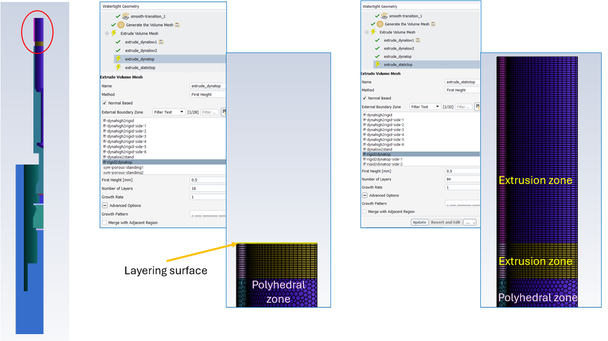
Extrusion “extrude_dynatop” creates an extrusion for the upper outlet expansion zone.  This zone will move in rigid fashion in Fluent simulation.  The top surface of this extrusion will have layering.  Extrusion “extrude_statictop” is the extruded cell zone at the outlet.  This zone will contract or expand in height during the simulation per the position of the layering surface.

Rod Pump Simulation Setup in Ansys Fluent

Fluent flow simulation setup specifies transient solver, single phase, oil material properties, and boundary conditions.  For this simulation, dynamic mesh is used to move a portion of the mesh.  The inlet and the outlet are specified as zero-gauge-pressure boundaries.  The walls are specified as no-slip walls.  Traveling and stationary valves are modeled as porous media cell zones.

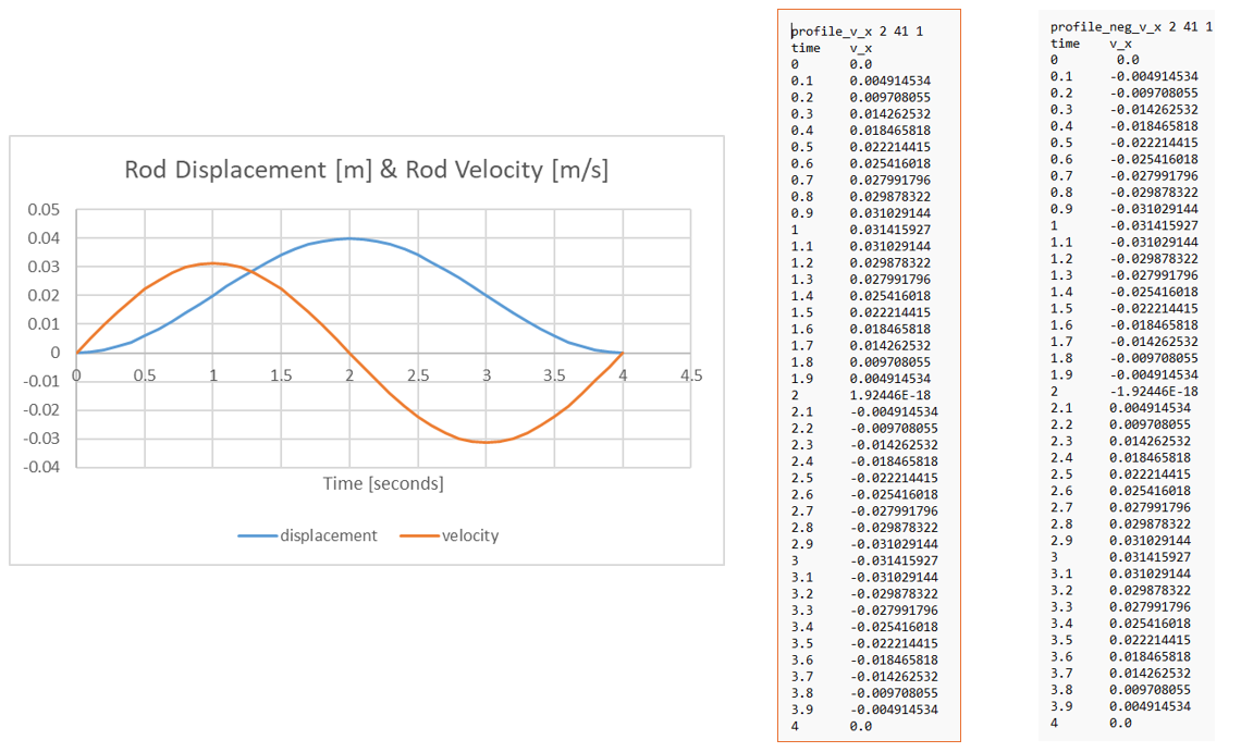
Velocity Profiles: The transient velocity of the rigid zones is needed.  This can be generated with a spreadsheet which is used to generate a transient table.  It is helpful to define the displacement equation and then to take the time derivative of that equation to obtain the velocity.  Another table should be generated which is the negative velocity.  The tables can be read into Fluent via the Profiles tool or via the TUI with /file/read-transient-table.  In both files there is a header.  The first line of the header contains the name of the profile, the number of columns, the number of rows, and the periodic flag.  If the periodic flag is 1, then time-periodicity is enforced.  The first and last rows of the profile should have the same dependent-variable value.

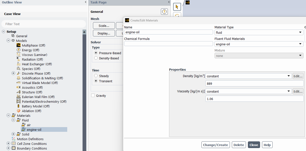
Models and Materials: A transient, single-phase, iso-thermal, single-species simulation is to be performed. Engine oil from the Fluent material database is used to model the fluid.

Cell Zone Conditions: Engine oil material is applied to all the cell zones.   Porous media is applied to the cell zones that represent the valves.

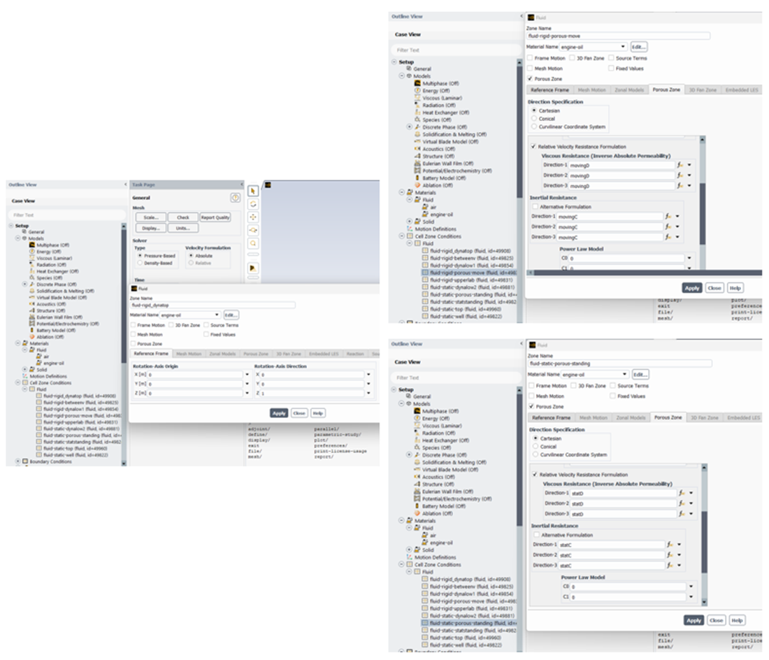
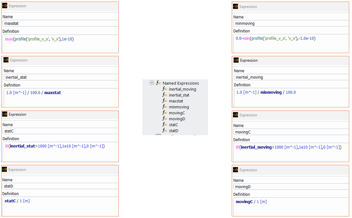
Named Expressions: The porous media cell zones include expressions for the viscous and inertial resistance coefficients to represent opened or closed valves. The goal for the valves is to represent a solid blockage or a low resistance object depending on the vertical motion of the rod pump in the simulation.  The stationary valve should introduce very high resistance when the plunger is moving downward.  Conversely, the traveling valve should introduce very high resistance when the plunger is moving upward.  Both values should introduce very high resistance when the magnitude of the traveling components’ velocity is near zero.  Expressions can be used to set these resistances based on the velocity from the transient table.  The left column lists expressions used for the stationary valve, and the right column lists expressions used for the traveling valve.  A max or min function is used to force a positive velocity variable.  Then a reciprocal of this velocity is found to make the resistance inversely proportional to the velocity.  A conditional statement follows to force either a very large inertial resistance value or a zero-resistance value. The final expression creates the viscous resistance by modifying the unit.

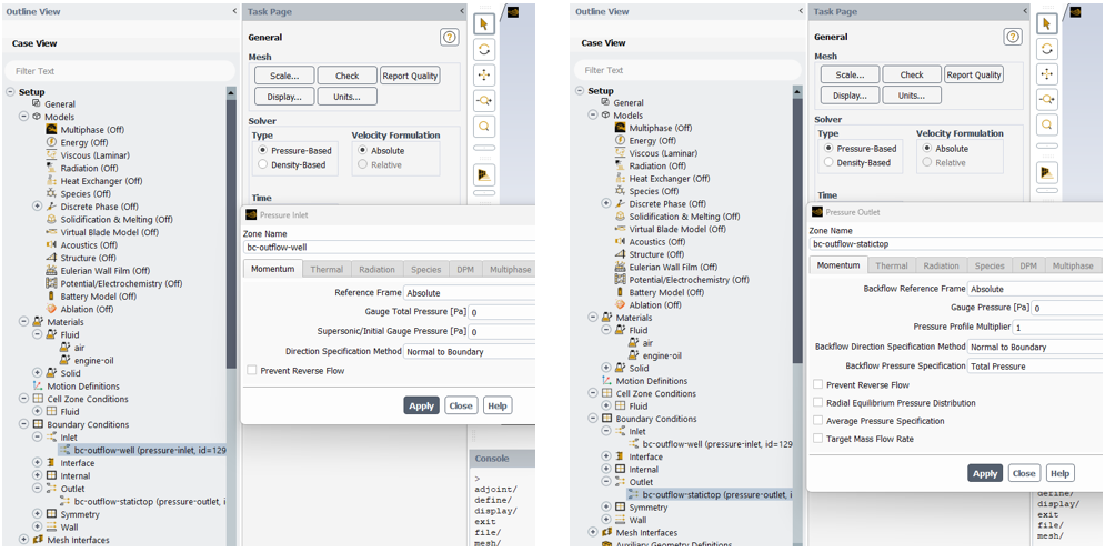
Face Zone Conditions: Boundary conditions include symmetry, walls, and pressure openings.  The settings for the pressure inlet and pressure outlet are shown below.  Both use a gauge pressure of zero.

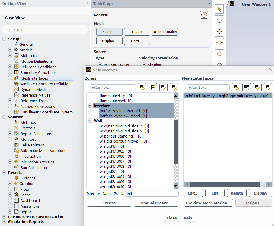
Mesh Interfaces: The lower extrusion extended to a polyhedral face; however, the mesh is not conformal here.  Therefore, the Mesh Interferences tool is needed to generate a mesh interface.  The two non-conformal faces are selected, and Create is selected to generate the Mesh Interface zone.

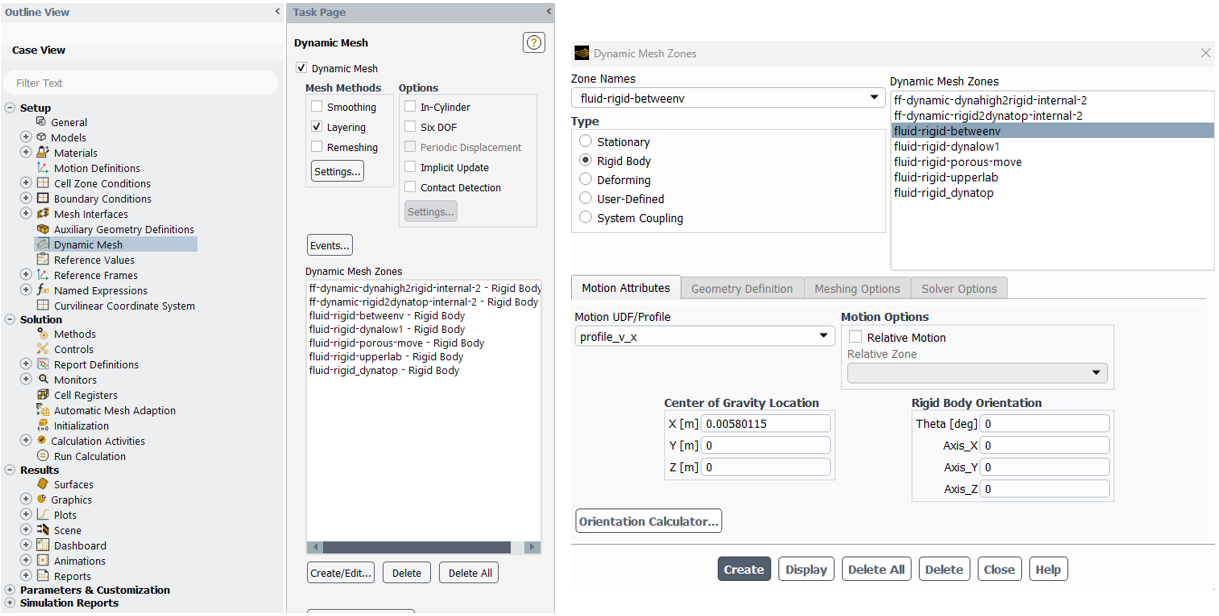
Dynamic Mesh: Multiple Dynamic Mesh Zones are needed to set the motion of the traveling components and to set the layering at the face zones between moving and stationary cell zones.  The Dynamic Mesh module is activated and all Mesh Methods and Options are deactivated except for Layering.  All the Dynamic Mesh Zones listed below use the “profile_v_x” Motion Profile.

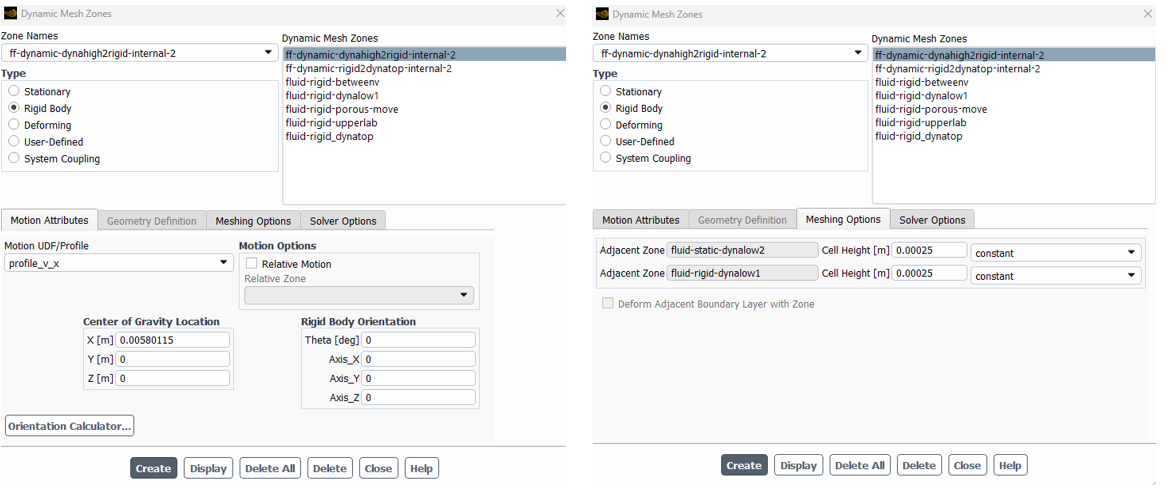
Dynamic Mesh: The two face zones (ff-*) where layering occurs are also specified with the “profile_v_x” Motion Profile; however, they are also both specified with Cell Height values in the Meshing Options tab.  The value is set to be consistent with the mesh size near that layer zone

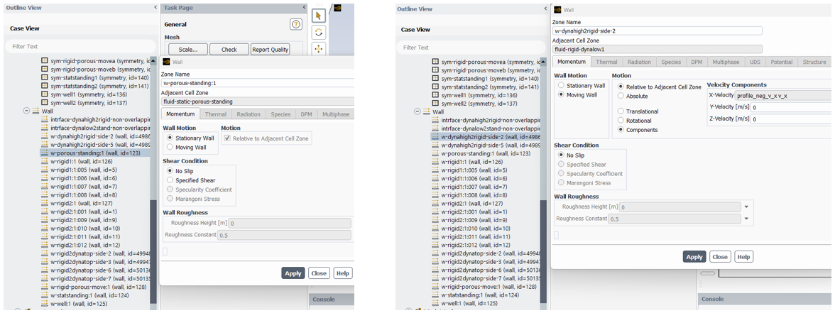
Face Zone Conditions: When the Dynamic Mesh module is activated and includes fluid zones specified with rigid motion, there may be wall face zones attached to the cell zone that will unintentionally “move” because wall face zone Wall Motion is stationary and relative to adjacent cell zone by default.  For example, walls of the plunger move with the rigid fluid body; however, the walls of the hole need to have zero velocity even though they are adjacent to a moving rigid fluid cell zone. In these cases, the Wall Motion should be specified as “Moving Wall” and should use a Velocity Components specification which uses the profile of the negative of the plunger velocity.

Post-processing: A Mass Flow Report Definition is employed to monitor and record the mass flow rate through inlet and outlet surfaces. A contour plot can be employed to display the velocity of the walls to confirm correct movement.  A contour plot of fluid velocity on the symmetry faces can be employed to visualize the motion of the fluid.  Animations can be employed to visualize transient contours. A mirror image is set through the Views module.

Fluent Simulation Results

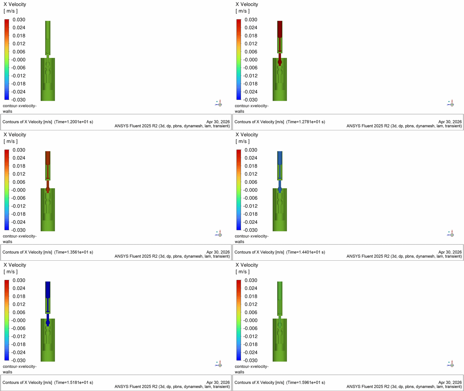
The animation of the wall velocity distribution shown below illustrates the motion of the plunger as well as the zero velocity of the stationary walls (in green).

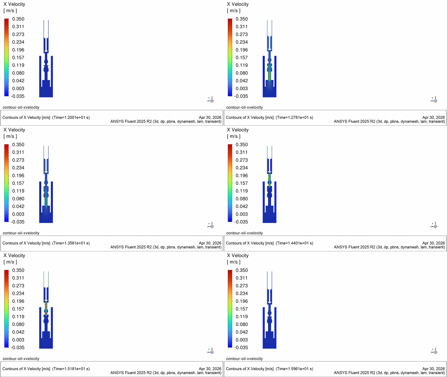
The animation of the fluid velocity is shown below to illustrate the motion of the fluid as a function of the motion of plunger and as a function of the resistance of each valve.

A key result is the flow rate through the pump.  The result below shows the transient flow rate through the pump over two cycles.  A time-average flow rate can be calculated from these results. As the plunger moves upward (8 seconds < time < 10 seconds) the traveling valve is closed and the plunger lifts fluid up and out through upper outlet. As the plunger moves downward (10 seconds < time < 12 seconds) there is negligible flow through the stationary valve which results in negligible flow through the inlet.  As the plunger moves downward it also displaces fluid volume above the stationary valve which pushes a small quantity of flow up through the outlet.

Rod Pump Simulation Setup Video

The following video walks through the simulation setup from the geometry to meshing to flow solver.

Improve Rod Pump Performance With CFD

Rod pump design seeks to reach product requirements which includes robustness to down hole conditions.  SimuTech Group’s fluids team helps engineering organizations use Ansys simulation tools to evaluate complex problems to make more confident design decisions earlier in development.

Whether you are working on an oil pump or a blood pump SimuTech Group can help you build stronger simulation workflows with Ansys Computational Fluid Dynamics tools such as Fluent.

Talk to a CFD Expert