Thermal Simulation and Temperature Feedback for Electric and Electronic Applications

In this blog we’ll discuss thermal simulation of electric and electronic applications and some of the considerations and assumptions, then show examples of how and why these things matter. But first, let’s ask why engineers would want to run thermal simulations for electric applications and then we’ll talk about temperature feedback.

Why Perform Thermal Simulation?

There are few reasons to run thermal simulations for electric applications:

• Heating is the main reason for component failure: It’s known that heating of electric applications is a major concern. Material failure (solder melting, wire insulation damage, demagnetization, etc.) and structural failure from thermal expansion and cycling are some examples of failures from electronics generating heat.
• Safety Concerns: Overheating components may pose danger to humans or exceed regulation limits.
• Performance Accuracy: Since material properties are temperature dependent, it can be important to simulate the heating to better analyze the application. Neglecting the heating can change the analysis results. For example, elevated magnet temperatures can reduce or change the performance of electric machines (motors). Or electric current heating aluminum conductors, raising the temperature from 20°C to 60°C raises the electrical resistivity and power by ~17%. Neglecting that change may be problematic for some applications.
• Desired Heating: Some applications have the heating as the main goal, such as induction heating applications, resistive heating, and others. For such applications, thermal simulation is done to understand the performance of the process. Another example is where the heating is affects for another process, such as material expansion.
• Equipment sizing: Often cooling equipment is required to maintain safe temperatures and the size and capacity of the cooling equipment (fans, pumps, etc.) is determined based on the heating results.

It is also not uncommon for more than one reason to be present in an application.

What is Temperature Feedback?

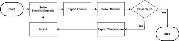
When running a thermal simulation, the heat loads (power densities) are supplied from an electric simulation. For example, Ansys Maxwell may be used for simulating current in a conductor, then feeds Ansys Mechanical or Ansys Fluent the heat load for a thermal simulation. An important question is whether the resultant temperature affects the original heat load and should it be sent back to the electric simulation for an updated heat load.

Sending the temperature from the thermal solver back to the electric solver is called feedback.

Does Temperature Feedback Matter?

Yes, it does.

But sometimes it can be ignored.

As with all simulations, the engineer must have some understanding of the application and physics and to make assumptions.

Temperature feedback matters because the material properties are always temperature dependent. This means that as the material heats, the material properties change, and the heat loads will change as a result.

Generally, temperature feedback provides a more accurate representation of the physical application. However, including temperature feedback means longer simulation times, often significantly more solve time and setup time.

The question of whether it matters comes down to the specific application and level of accuracy the engineer wants.

What Types of Temperature Feeback or Coupling are There?

There are different types of applications when it comes to temperature feedback, such as the following:

• Low heat, low temperature rise, and/or low material property temperature dependence. For those applications it’s better to ignore temperature feedback as the marginal increase in accuracy is not worth the setup effort or simulation time increase.
• Low Temperature gradient applications. For those applications it’s better to ignore temperature feedback as well. However, in some applications where the temperature rise is not negligible but relatively uniform, the initial temperature can be assumed for a better estimate of losses.

• Simple Feedback. This type of feedback returns the final temperature (steady state temperature, or last time step of a transient simulation) to the electric simulation. This is done in an iterative matter until a convergence criterion is met. This type of feedback is usually appropriate for steady state applications for simple transient simulations (slow transient problems with linear material property temperature dependence).

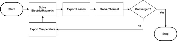
• Transient Simulation. This type of simulation returns the temperature every time step or every n^th time step to ensure the proper update of the material properties. These types of simulations are more costly as they require the electric and thermal simulations and data mapping to occur every time step. These types of simulations are used for highly transient applications and when the material properties change significantly and rapidly or when the temperature dependence is highly non-linar. A famous example is steel induction heating. Those applications usually heat steel from room temperature to ~1000°C in a few seconds, resulting in a rapid change in the non-linear magnetic properties, passing through the Curie point, and a large drop in electrical conductivity. Simple feedback will miss the massive changes that occur during the heat cycle.

Examples of Thermal Simulation

Copper Heating

In this example, 2D simulations of copper bus bars (leads) were made to show the effect of copper choice on losses and temperature. In these examples the frequency and current were held constant, but the wall thickness was changed. The losses were fed from Maxwell Eddy Current to Ansys Mechanical for a steady state thermal simulation, with temperature feedback to investigate the heating of the copper.

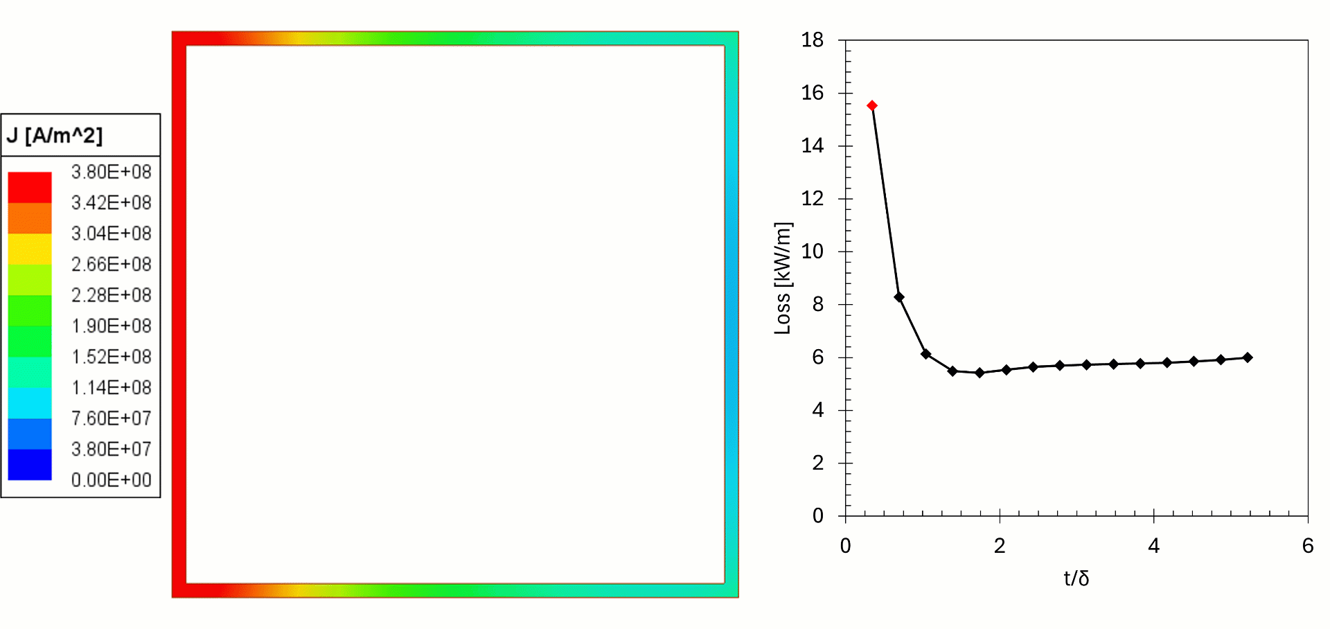
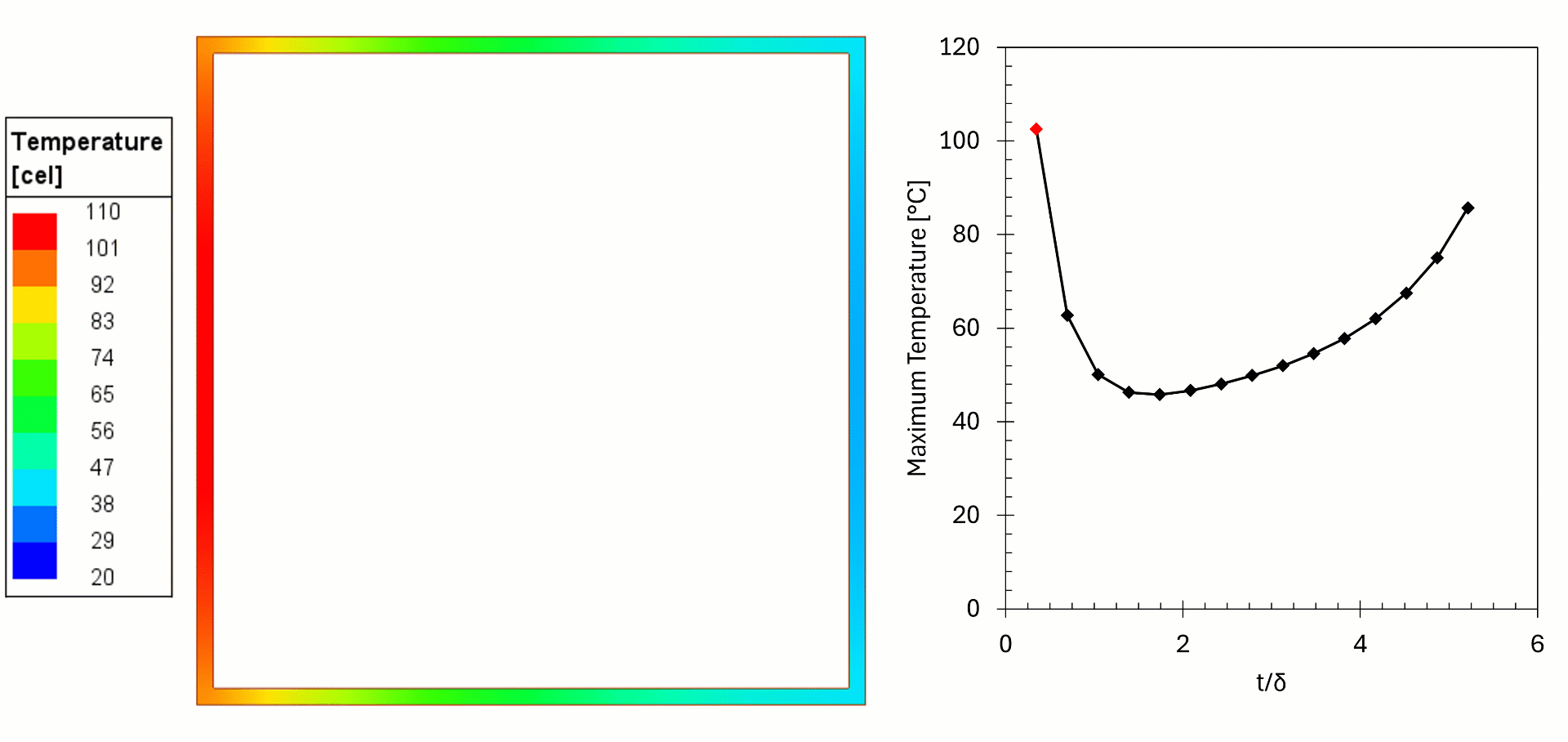
We can see from the results that for thin walls the losses in the copper are high, as the current flows in a thin cross-section, resulting in higher temperatures. For higher wall thicknesses the cooling surface is farther away from the current, resulting in higher temperatures. We can see that when t/δ>2 (δ is skin depth) the current density remains the same, but the power gradually increases, this is due to higher temperature of the copper. The effect is negligible in this example but can be problematic in other cases if not considered. The simulation shows there is an optimal wall thickness: too thin will increase the temperature and likely fail prematurely and too thick is costly and increases the temperature (in practice, commercially available tubes come in set thicknesses and custom sizes are expensive, thermal simulations give the designers better insights for the choice).

For machined copper coils the wall thickness can be controlled, and cooling channels can be machined to reduce the heating of the copper’s hot zones to improve coil life.

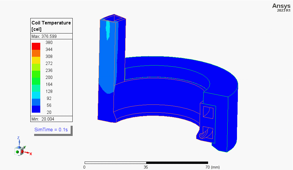
The image shows the heating of a coil designed for the hardening of a wheel-hub (simulated but not shown here). The bottom of the coil has a channel machined to reduce the temperature of the coil’s tip, which overheats due to the skin, end, and proximity effects. The simulation also shows the leads heat the most during the cycle, this is due to the proximity and skin effects and the low wall thickness (poor heat sink). Geometry courtesy of Fluxtrol Inc.

Steel Induction Heating

In this example we have a 2D axisymmetric induction heating simulation of a carbon steel cylinder. Steel heating is interesting because it is magnetic and when heated past the Curie point (~760°C) it becomes non-magnetic, while the conductivity drops. Due to the nature of the heating (high skin effect and fast heating rates, and significant difference in the loss distribution pre and post Curie point) the temperature is highly non-uniform, and the heat rate is highly temperature dependent.

This type of heating is common for heat treatment, such as hardening and tempering, and requires challenging and specific heat distributions to achieve the desired patterns. Accurately simulating the temperature is essential for these applications.

In this example we will show how transient coupling (using Ansys System Coupling) results compare to simulations with no feedback and simple feedback.

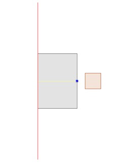
The image shows the geometry used for the simulations. Constant current and frequency of 10kHz were used. Temperature dependent electrical conductivity and temperature dependent non-linear B(H) magnetic properties were used.

The red line indicates the symmetry axis while the yellow line and blue point were used to plot temperature for comparison. The results for the yellow line are plotted for the last time step.

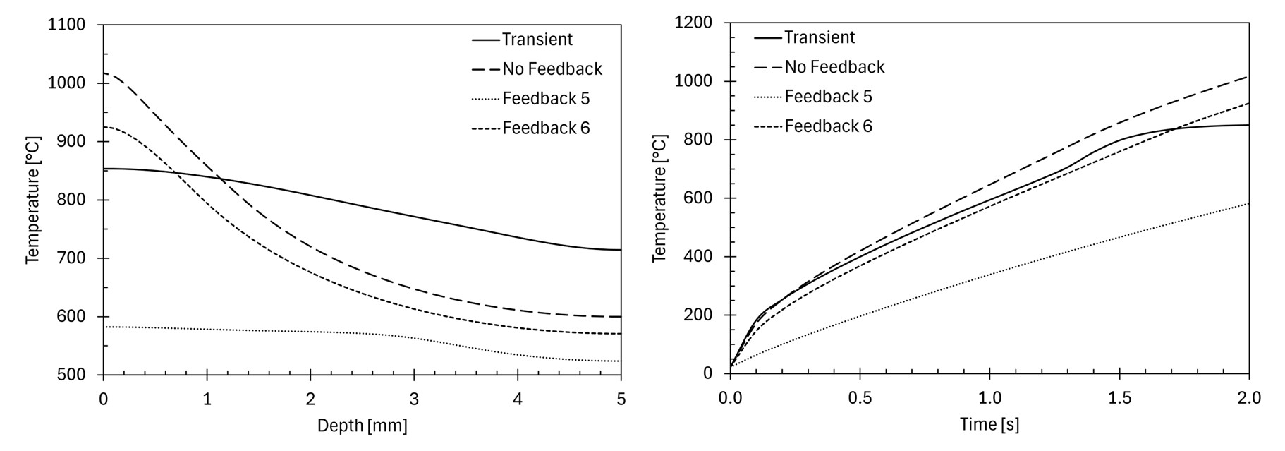
The two images show major variation in the temperature results when using different coupling methods. Using no temperature feedback will result in overheating due to the heat load being calculated on the magnetic steel, overestimating the results. Furthermore, we can see a more pronounced skin effect maintained at the end of the cycle.

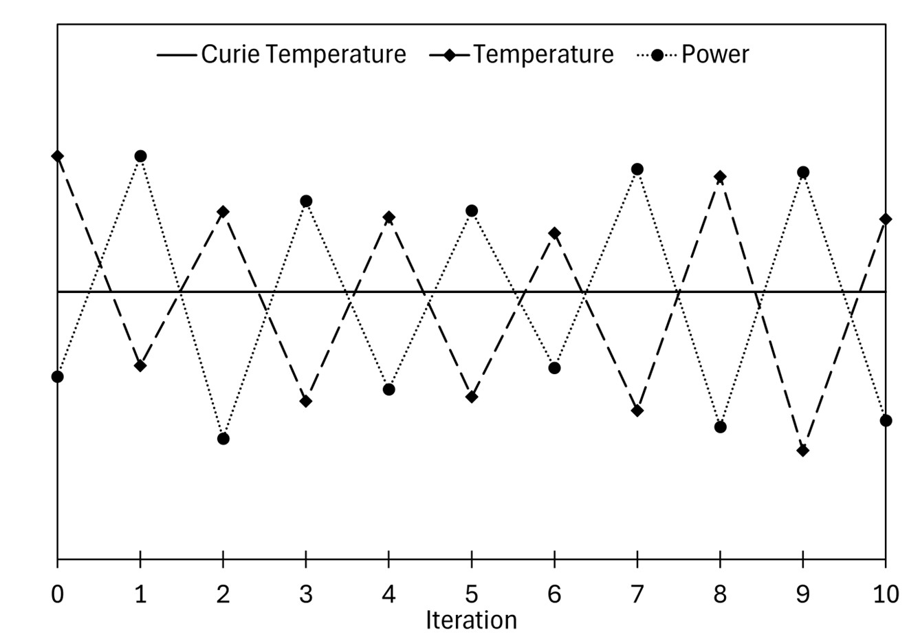
Another behavior that is shown is the vast difference between the 5th and 6^th iterations of the simple feedback coupling. This is interesting because when Maxwell is fed temperatures above the Curie point, the calculated heat is lower with lower skin depth, resulting in temperatures that are below the Curie point, which will result in higher heat rates, and so on. This coupling scheme will not converge and will continue to oscillate in temperature around the Curie point. In fact, it will not even produce the same two oscillating results, so the simulation is unacceptable. The image below shows, in a simplified way, how the temperature and power oscillate every iteration.

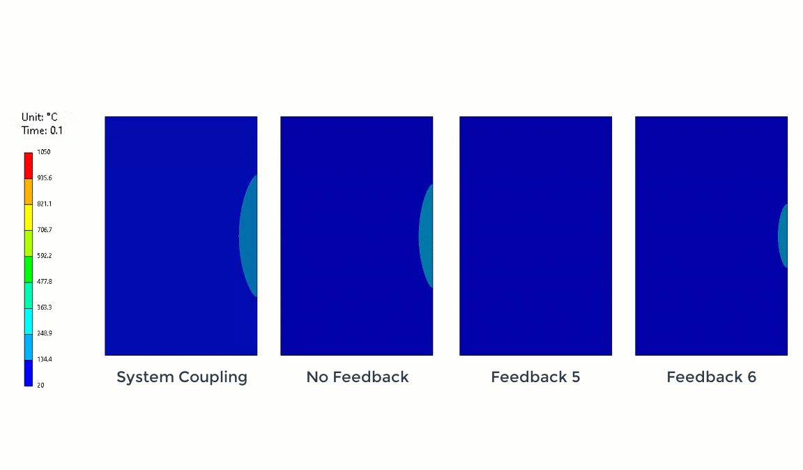
This image shows the temperature contour during the heat cycle for each coupling method.

In this example, the simulation was solved to 2.0s with 0.1s time step. Here’s how those simulations look:

Coupling Method	# of Maxwell Solves	# of Mechanical Solves	Simulation Conclusion
No Feedback	1	1	Not a good simulation
Simple Feedback	Diverges	Diverges	Diverges, bad simulation
System Coupling	20 minimum	20 minimum	Good simulation, expensive.

If the induction heating application heats the steel to low temperatures and does not approach the Curie point or if the workpiece is non-magnetic (stainless steel, brass, etc.), then simple feedback may be an acceptable assumption. It is important for the engineer to understand the physics and make an assessment for the acceptability of their assumptions.

Thermal Simulation in Conclusion

Thermal simulation of electrical and electronic applications is a popular and important engineering tool for understanding heat generation, predicting temperatures, and optimizing applications. Thermal simulations may require temperature feedback. It is important for engineers to be aware of their applications’ needs and assess what type of thermal feedback, if any, they want to do.