In this blog, I demonstrate how to compute the winding inductance using Flux Linkage and Current results from the Magnetic Transient Solver in Ansys Maxwell. The Ansys Maxwell Magnetic Transient Solver accounts for eddy effects in field calculations, and I will show an easy method to compute winding inductance using the results of Flux Linkage and Current.
In reality, inductance is non-linear and depends on frequency and temperature. The incremental (differential) inductance is the actual inductance at a given frequency, operating point, and temperature. The winding inductance first changes along the magnetizing curve, starting from zero current and flux, and then changes around the hysteresis loop. In the region before the “knee” of the magnetizing curve (the practical region in transformers and rotating machines), the apparent inductance can be used to approximately linearize the inductance, and simulators would give reasonable results, depending on the application. After the “knee” of the magnetizing curve, in the saturation region, linearizing inductance would not yield accurate results in simulation. Sometimes air gaps are used in cores to linearize the inductance, but this would reduce the flux for a given MMF without the air gap, and higher winding losses would incur.
Many useful engineering applications do not need a nonlinear model if the linear model is good enough. The question of what the acceptable error is in the application should be considered and answered.
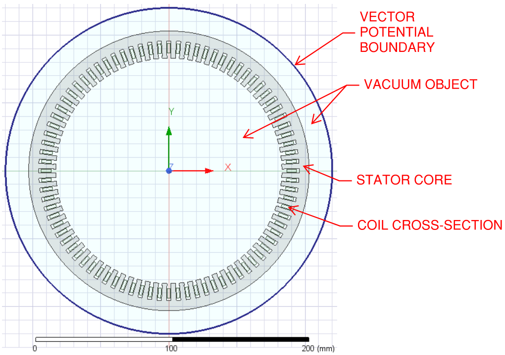
Maxwell Model Setup
Mesh operations were applied to the core to obtain accurate results. Three-phase sinusoidal excitation of one amp was applied to the windings. The time step used was the electrical period divided by 1000.
Magnetizing Curves and Hysteresis Loops
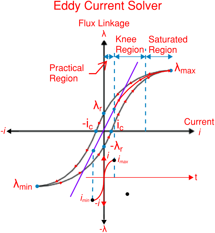
The magnetizing curve of a non-linear magnetic material is developed by applying excitation starting from zero excitation and increasing in one direction, say the “positive” direction, up to a maximum point in the saturated region where the slope equals the inductance with an air core. Magnetizing curves can be represented as a Flux Linkage and Current relationship or a Magnetic Flux Density and Magnetic Field Strength relationship, and both are directly related and scaled versions of each other. Both curves have the same shape and characteristics.
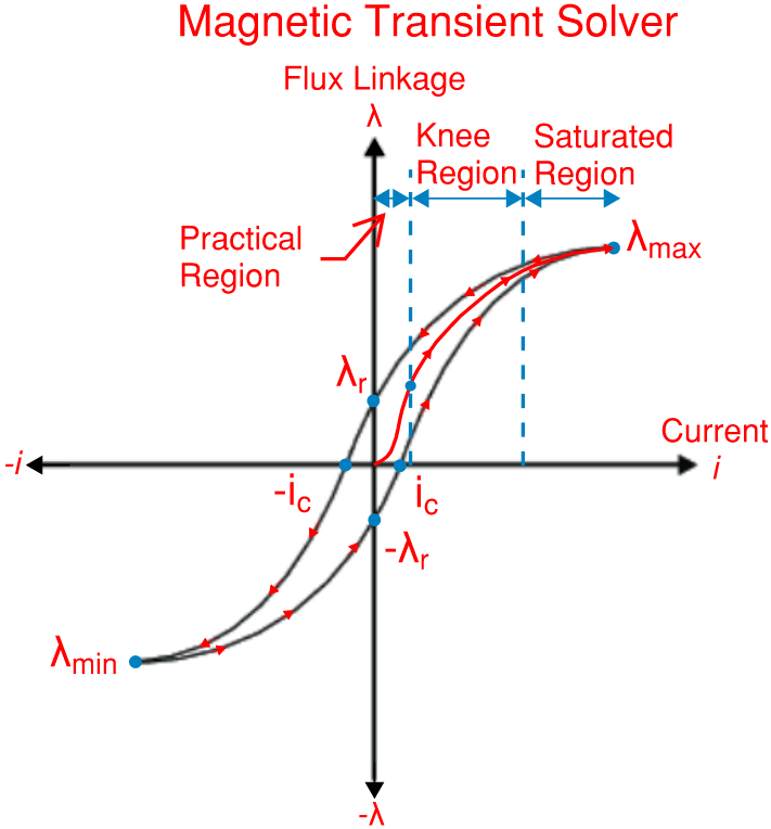
The magnetizing curve can be divided into three distinct regions as follows:
(1) Practical Region: optimum performance where inductance is high for a small excitation current, winding loss is low, and induced voltage, current, and torque are high.
(2) Knee Region: performance declines and inductance decreases.
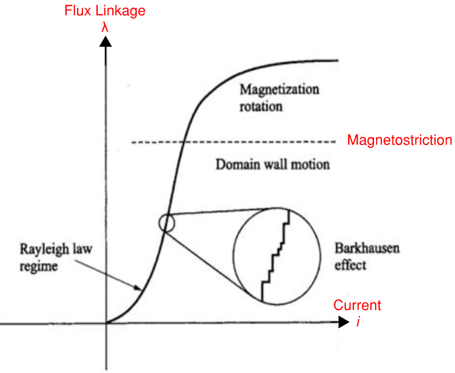
(3) Saturated Region: inefficient performance where inductance is equal to the inductance of an air core inductor. Applying a large increase in current excitation is not justified because it does not result in a large increase in flux linkage gain, as in the practical region, and winding loss is increased with current squared. Also, a saturated core contributes to higher harmonics in the winding currents and air gap flux density (rotating machines), noise (humming), and vibration in the core due to the Barkhausen effect and magnetostriction, and harshness, which is associated with noise and vibration.
Magnetostriction is the change in volume of a saturated core as magnetic domain walls expand, allowing the domains to align with the applied field. The domain walls boundaries expand (domain wall motion) or change structure (magnetization rotation). The Barkhausen effect is due to rapid changes in magnetic domain alignment and is stronger in the saturated region. The figure below shows that the magnetizing curve is not smooth.
Magnetostriction is not desired in rotating machines and transformers. However, some actuators and transducers use magnetostrictive material to convert magnetic energy into kinetic energy.
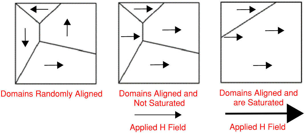
Magnetic wall boundaries divide the magnetic structure into domains where magnetic dipoles in each domain are aligned in the same direction, while magnetic dipoles are aligned in other directions in other domains. When a magnetic field strength H, a function of current, is applied to a magnetic material, the magnetic field permeates the material and aligns all the magnetic domains in the direction of the applied field. In the non-saturated, practical region, the magnetic domain wall boundaries expand and contract as the applied field changes direction, and the domains realign with the field, but the structure of the wall boundaries does not change significantly. However, under saturation, the structure of the magnetic domain wall boundaries changes (reshapes) significantly, or boundaries are removed during the alignment of the domains with the applied field (larger than necessary and without benefit).
The magnetizing curve does not follow the same path when the current is reversed at any operating point because the magnetic material has “memory”, and this phenomenon is called “Hysteresis”. Flux Linkage remains, “Remnant Flux”, in the core after the excitation is brought to zero from one direction. Applied current excitation, “Coercive Current”, in the opposite direction is required to bring the flux to zero.
The deviation from the original path is smallest in the practical region (smallest losses) and largest in the saturated region (largest losses). Magnetic material contribute to power losses equal to the area of the loops formed by hysteresis over one period of excitation.
The apparent inductance at the operating point is used to linearize inductance in the Eddy Current solver, and in general in any other frequency domain, steady state solver that uses AC waveforms. There is only one inductance in this type of solver, whereas in the Magnetic Transient solver, there is also an incremental inductance.
Flux Linkage vs. Current
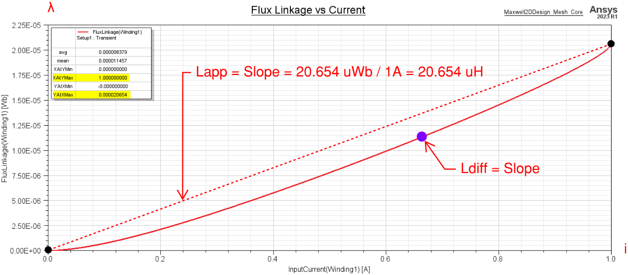
Flux Linkage vs Current (from zero to maximum) is plotted below. The apparent inductance is equal to the Flux Linkage divided by the Current with respect to the maximum operating point.
Incremental Inductance vs. Current
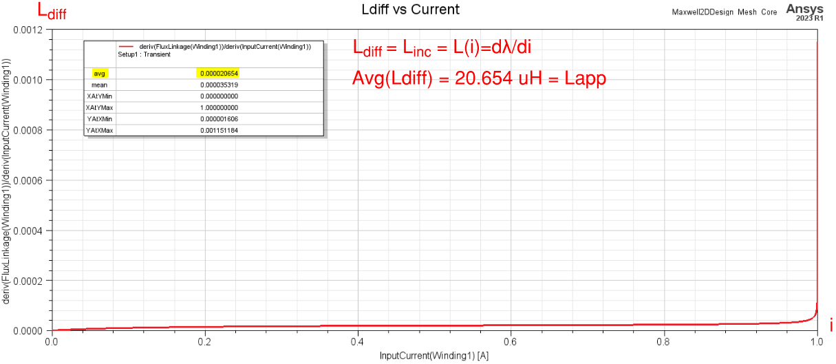
The incremental inductance, or differential inductance, is the derivative of the Flux Linkage vs Current plot. We see in the results below that the average incremental inductance equals the apparent inductance.
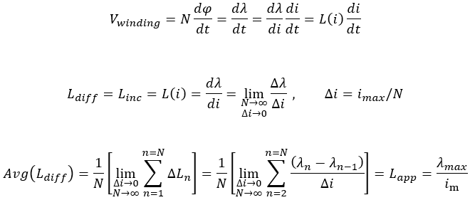
Flux Linkage vs. Current Analysis
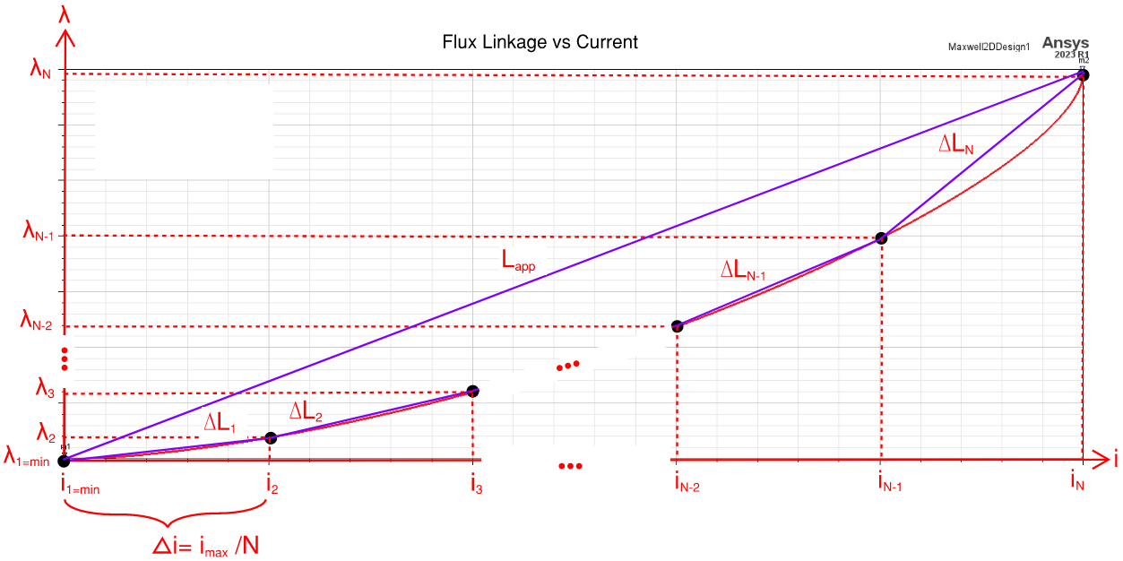
Below is an analysis showing how the average of the incremental inductance equals the apparent inductance.
Working on winding inductance or electric machine design? SimuTech Group’s Maxwell training course covers setup, solving, and post-processing for low-frequency electromagnetic simulations. For a broader look at electric machine workflows, see our guide on electric machine design in Ansys. Contact us to discuss your electromagnetic simulation needs.