How to Estimate the Thermal and Electrical Properties of TECs for AEDT Icepak Modeling

Introduction to Ansys Icepak TEC Modeling

In many thermoelectric cooler (TEC) datasheets, the device-level performance curves (e.g., Q̇_c vs I, V vs I) are provided, but the underlying temperature-dependent coefficients required by Ansys Icepak for the different material properties are not. This blog outlines a practical workflow for Ansys Icepak TEC modeling: estimating those coefficients from manufacturer curves and then validating them with a simple Icepak model. The objective is to obtain a calibrated set of properties that reproduces the datasheet behavior over the operating range of interest. Detailed information about the internal construction is also helpful, since it can significantly improve the accuracy of the estimation.

Thermoelectric Coolers in Electronics Cooling

Thermoelectric coolers play a critical role in electronic cooling because they provide solid-state, compact, silent operation, and highly controllable heat pumping without moving parts or refrigerants. By using the Peltier effect, TECs can actively transfer heat between two locations even below ambient temperature, enabling precise temperature regulation of sensitive electronic components such as lasers, CPUs, sensors, and power electronics. This capability is especially valuable in applications where reliability, low maintenance, fast thermal response, and operation in any orientation are required, or where traditional air or liquid cooling solutions are impractical. As power densities in modern electronics continue to increase, TECs offer an effective complementary cooling technology to maintain performance, stability, and device lifetime. In this blog, we will address how you can estimate the thermal and electrical properties of a TEC so you can more accurately model TEC performance in Ansys Icepak.

Governing Equations for TEC

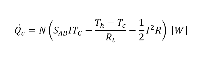
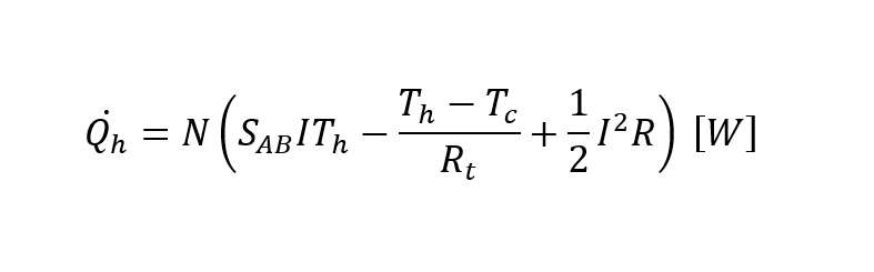
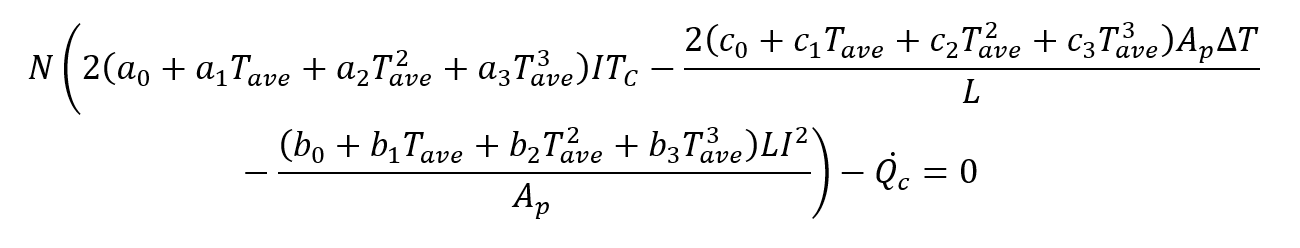
TECs work based on the Peltier effect, in which the main outputs are the heat pumped at the cold side (Q̇_c) and the total heat dissipated at the hot side (Q̇_h), and the main inputs are the current (I) and the voltage (V). The TEC model is governed by three effective parameters: the Seebeck voltage (S_AB), the electrical resistance (R), and the thermal resistance (R_t). Q̇_c and Q̇_h have their own equations based on the number of thermoelectric couples (N), S_AB, R_t, R, the temperature at the cold side and hot side (T_c and T_h), and the current, as shown in the two equations below:

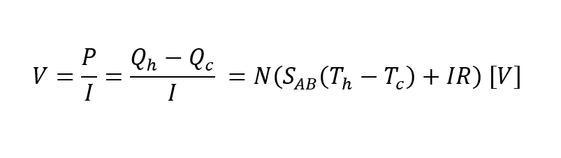
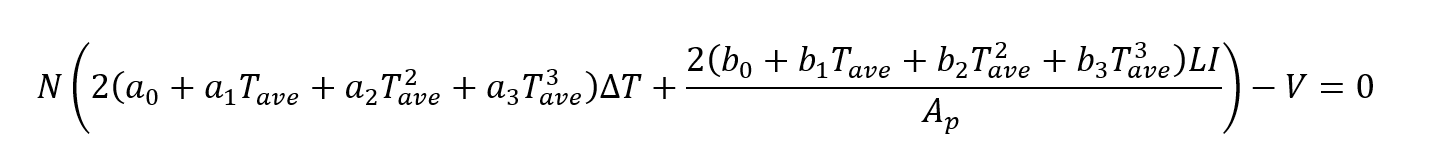
In addition, the voltage required by the TEC can be calculated as:

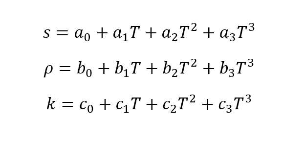
Furthermore, S_AB, R_t, and R are related to the Seebeck coefficient, electrical resistivity, and thermal conductivity as shown in the equations below:

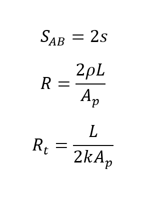
Where s is the Seebeck coefficient (V/K), ρ is the electrical resistivity (Ohm-cm), k is the thermal conductivity (W/cmK), L is the pellet height (cm), and A_p is the pellet cross-sectional area (cm²). L and A_p are related through the G-factor, defined as A_p/L. These material parameters are required by Ansys Icepak TEC models, and since they typically vary with temperature, Icepak allows you to enter polynomial coefficients instead of a single constant value, as shown below:

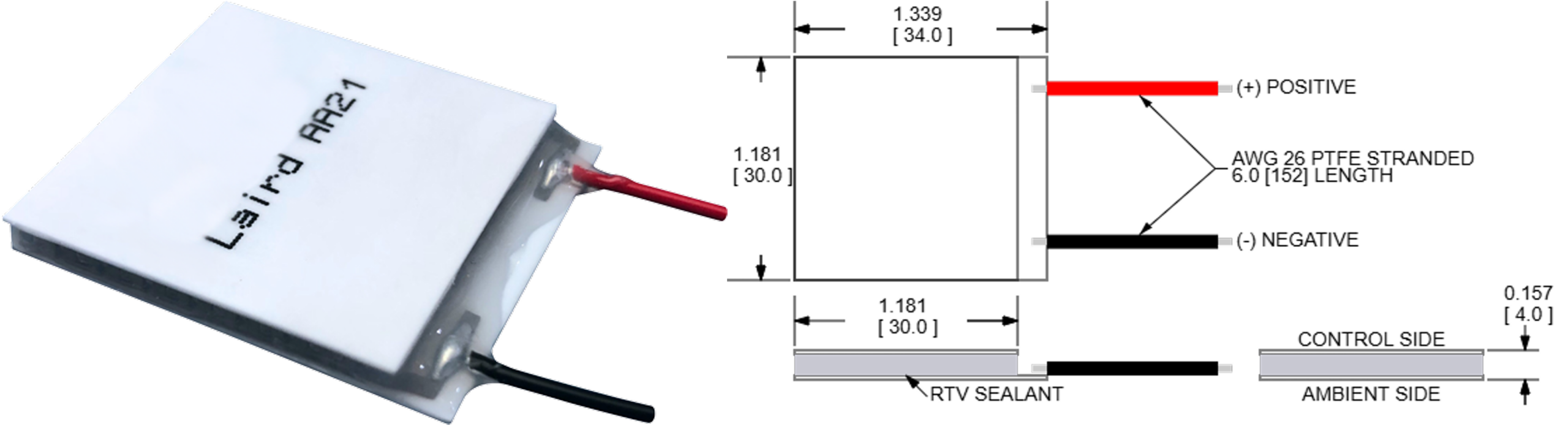
In other words, we can use up to twelve different coefficients for the TEC material properties, which must be estimated from the manufacturer’s performance curves. For this blog, we will estimate the coefficients for the TEC HiTemp ETX Series ETX1.6-12-F2-3030-TA-RT-W6 manufactured by Tark, using the characteristic curves available in the datasheets. A picture of the TEC used for this blog is shown in Figure 1.

Before we continue with the methods to estimate these coefficients, I will explain how to add a TEC in AEDT Icepak.

Ansys Icepak TEC Toolkit in AEDT

The user can model and run a simulation with a TEC by using the TEC Toolkit in Icepak. You can access it by going to Icepak in the Toolbar → Toolkit → Modeling → Thermoelectric Cooler.

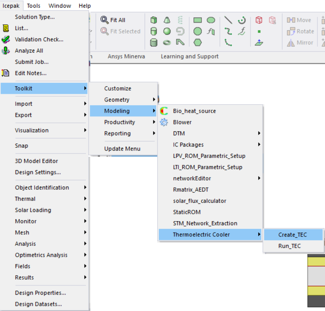
At this point, we have two options: Create_TEC and Run_TEC. Before we run anything, we need to create the TEC, so I will explain this first.

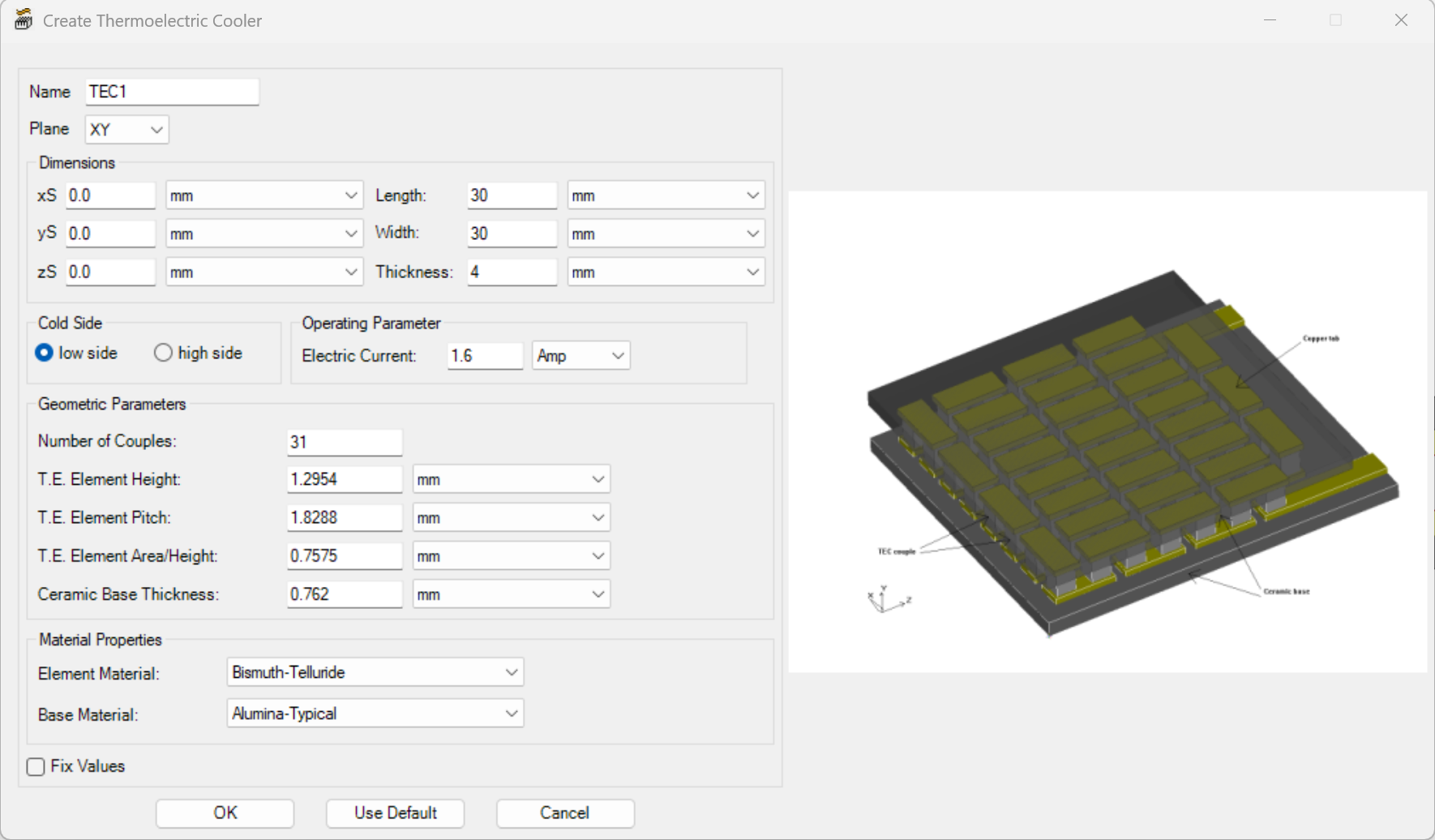
When you click Create_TEC, a new window will open that allows you to modify all the dimensions of your TEC. Most of the time, the only available information about the TEC is its length, width, and thickness. Based on the performance curve, we can also estimate the average current value at which the TEC will be working for our system. For this demonstration, we set the length and width as 30 mm, the thickness as 4 mm, according to Figure 1, and the electric current as 1.6 Amp. For the other variables, the default values were used.

Note: Keep your units consistent with the toolkit inputs. The coefficient equations are derived from pellet-level relations that assume a coherent set of base units. If your CAD model uses mm, be sure to convert L and A_p consistently when estimating material property coefficients, which have units of cm.

Now that we have created the TEC, we can run the TEC. When you first open the Run_TEC tool, it will show you a section where you can add the different coefficients to account for temperature dependency for the Seebeck coefficient, electrical resistivity, and thermal conductivity. You also have to enter the correct number of TEC couples and G-factor that were used when you created the TEC. After you enter the values, you can save them to be used in future simulations. For instance, for a new run in which you want to run the TEC at a different current, you can load the property coefficients, change the operating current, and run the case with the new operating current. These are the steps we will follow to validate the estimation using a simple Ansys Icepak TEC model.

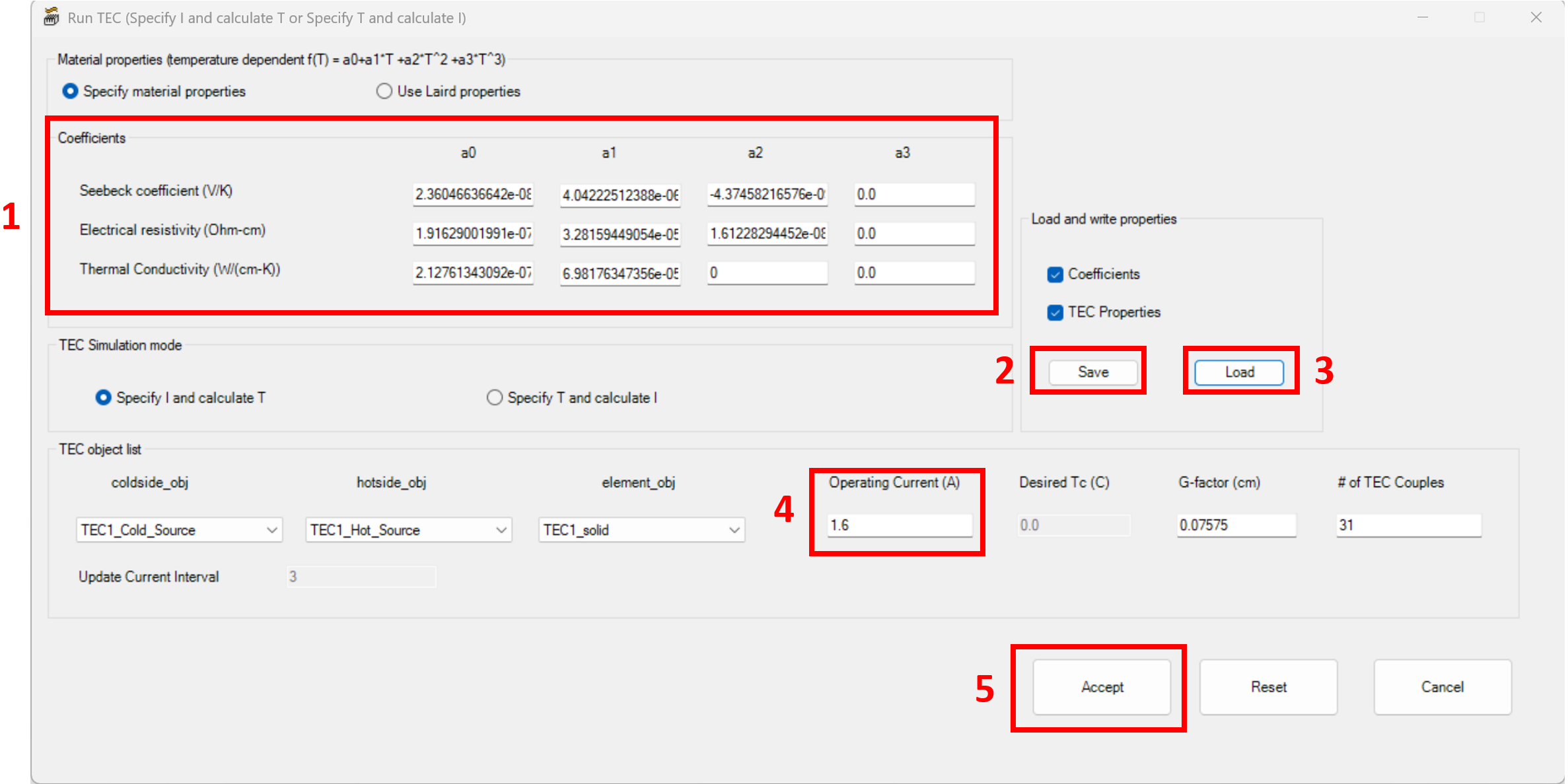
Note: While the simulation is running, it is not recommended to close this window since closing it may stop the simulation or create problems when the simulation finishes and saves the results.

Now that we understand how to define the TEC geometry and run the TEC macro, we can dive into the process of calculating the material-property coefficients. In this blog, we will calculate eight coefficients: three for the Seebeck coefficient, three for the electrical resistivity, and two for the thermal conductivity.

Coefficient Estimation Method

We will follow a series of steps that are summarized in the list below. These steps are based on how the Icepak TEC Toolkit is parametrized.

1. Choose T_h and the ΔT range that matches your application. Sometimes only one T_h is available, but the estimation gets better if we have different curves for different T_h.
2. Digitize curve points. From Q̇_c vs I and V vs I plots at two or more ΔT values according to the range that you are expecting the TEC to operate. Extract two or more points for each curve.
3. For each point, we can compute T as T_ave=(T_h+T_c)/2 to evaluate the material properties.
4. Choose the number of points to match the number of unknowns. Start with reduced polynomial order if you have difficulty solving the system with the full twelve variables.
5. Build the system of linear equations, using the Q̇_c and V expressions (one equation per point).
6. Solve for coefficients with a linear iterative solver using an external tool (e.g., Python).
7. Validate the coefficients in Ansys Icepak under the same boundary conditions and compare the results against the Q̇_c and V performance curves from the manufacturer.

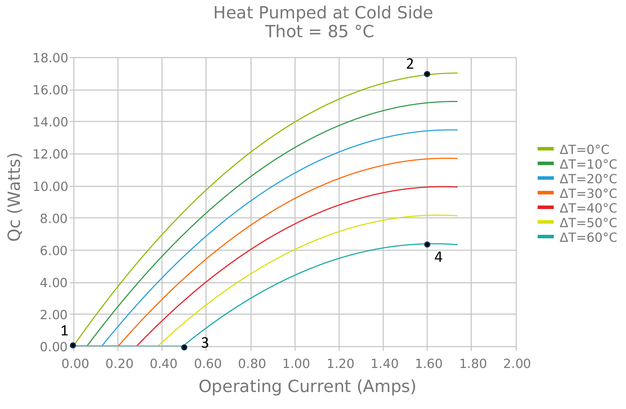
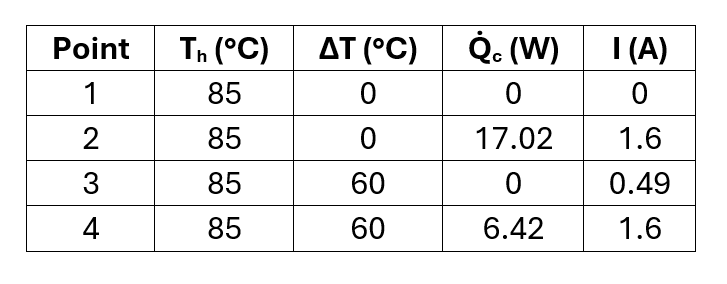
As an example, we are going to apply the steps mentioned above to characterize the material properties of the ETX1.6-12-F2-3030-TA-RT-W6 TEC. To estimate the coefficients, let’s first check the performance curve Q̇_c vs I (Figure 5). For this example, let’s use the extreme ΔT curves of 0 and 60 °C, and for the current, the minimum value and the value at 1.6 A for each ΔT curve. From this curve, we can get four points for our system of equations.

These four points are given in the next table:

We can do the same for the V vs I plot:

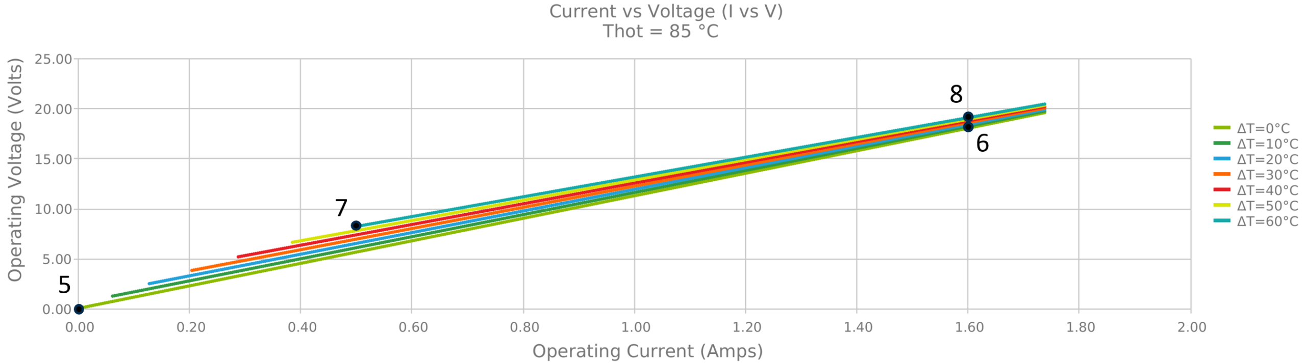
These four points are given in the next table:

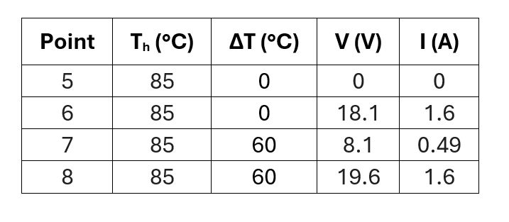
Using the four points from the Q̇_c vs I plot and the four points from the V vs I plot, it is possible to create a system of linear equations using each point with the following form for the Q̇_c values:

And the following form for the V values:

In which T_ave can be calculated as the mean temperature between the hot and cold sides (T_h+T_c)/2 or T_h-0.5ΔT, where ΔT= T_h-T_c and T_c= T_h-ΔT.

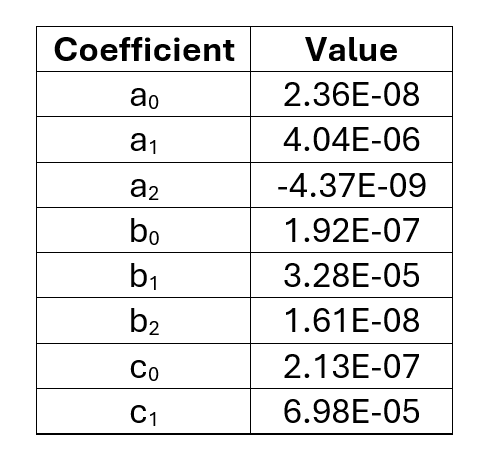
For this demonstration case, because we are using eight points, we will assume that a₃, b₃, c₂, and c₃ are equal to 0, so we only have eight variables. You can solve this system of equations by any means and obtain the values for each coefficient. The coefficients calculated by solving the system of equations with an iterative method in Python are shown in the table below.

Now that we have the coefficients, we can build a validation model in AEDT Icepak to verify these properties. The procedure described in this section is not a substitute for a detailed TEC model provided by the manufacturer; instead, it is a practical method to estimate and calibrate an Ansys Icepak TEC model so that the TEC performance matches the expected behavior in the simulation.

TEC Validation Using Ansys Icepak

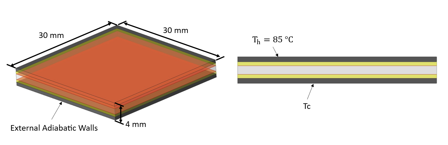
Using Create_TEC, we can create the TEC using the dimensions of our target device. For the boundary conditions, we set the top of the TEC to a fixed temperature of 85 °C, and we assign a fixed temperature at the bottom that can be adjusted to obtain different ΔT values across the TEC. Since only conduction is required for this validation, the air region can be removed. Figure 7 shows the validation model and the boundary conditions used.

Unfortunately, at the moment, there is no way to run a parametric analysis for a TEC because of the workflow required to execute the TEC Toolkit. Each run must be launched manually via Toolbar → Toolkit → Modeling → Thermoelectric Cooler → Run_TEC, and every time you need to reload the coefficients and manually set the operating current. Therefore, the TEC Toolkit was executed at multiple current values for two different ΔT conditions: 0 °C and 60 °C.

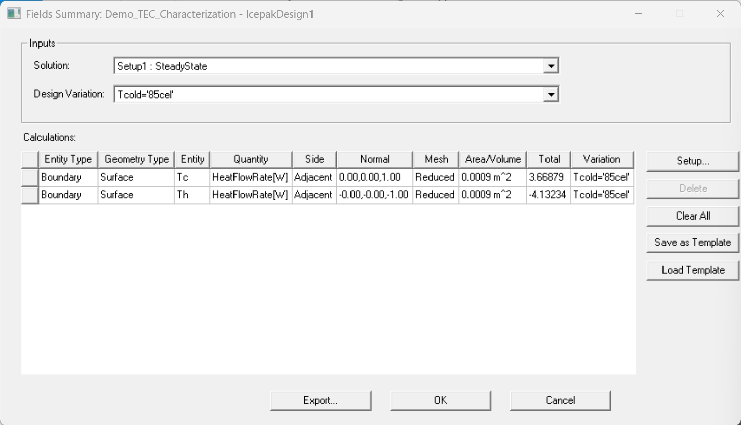
To postprocess the TEC results, we calculate the heat flow rates on the cold and hot sides using the Field Summary task. Based on these values, we can estimate the TEC voltage by computing the difference between Q̇_h and Q̇_c and dividing it by the applied current.

The results were compared against the manufacturer Q̇_c vs I plot and V vs I plot, which we used to extract the values for the estimation. The Q̇_c vs I plot and V vs I plot are shown in the figures below.

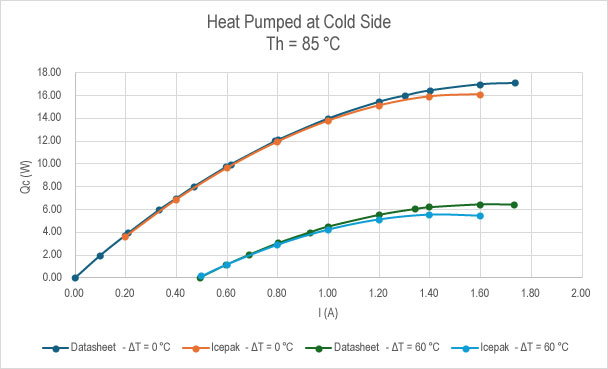
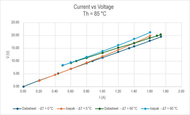
We can see in Figure 9 and Figure 10 that the TEC behaves as expected within the range of 0 to 1 A. However, it starts to deviate from this point when the current starts to increase. At this point, we can go back to the estimation and add more variables, or we can tune the coefficients or the G-factor so the behavior improves across the full current range.

For this specific case, we can also compare other variables or curves, such as Q̇_h vs I.

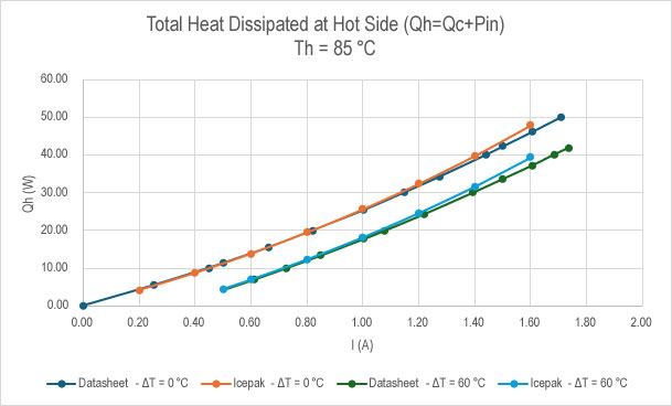
As you can see in the example above, this estimation is a first-order estimation, and we recommend validating TEC performance using a small model and then further tuning the coefficients to achieve the expected results.

Ansys Icepak TEC Modeling Conclusions

The estimation approach explained in this blog provides a first-order approximation of the material coefficients for the TEC model when full material data is not available. It is always recommended to improve the fitting only in the operating region you care about, prioritizing points near your expected current and ΔT. A global fit can sacrifice accuracy in the most important region.

Use multiple curves for cross-checking TEC behavior. Matching Q̇_c vs I is necessary but not sufficient; also compare V vs I and Q̇_h vs I if available. Always validate TEC behavior separately before system integration. The resulting coefficients are an effective first approximation of the material coefficients that replicate the performance; however, they may require further tuning for a better representation of the real TEC performance. They are not intended to replace detailed manufacturer construction information.

Bring Greater Confidence to Electronics Cooling Simulation

Accurate Ansys Icepak TEC modeling depends on more than entering values into a simulation tool. It requires thoughtful interpretation of datasheet curves, careful coefficient estimation, and validation against expected device behavior. With tools like Ansys Icepak, engineers can evaluate thermal performance, material behavior, cooling strategies, and system-level reliability before committing to physical prototypes.

For teams looking to improve electronics cooling workflows, SimuTech Group brings more than 40 years of simulation experience, deep technical knowledge, and top-level Ansys channel partner support to help bridge the gap between software capability and practical engineering application. Whether you’re building a first-order TEC model, refining thermal performance, or integrating cooling behavior into a larger electronics system, our experts can help you move from estimation to confidence.

Need help with Ansys Icepak TEC modeling or validating electronics cooling performance? Connect with SimuTech Group to discuss your simulation goals.