Polarization States for Zemax: Jones Calculus, Part II

Published: 06/11/2025

Updated: 04/28/2026

Jones Calculus Fundamentals and Notation in Zemax

Jones Calculus is a mathematical framework used in Optics to describe the polarization of light and how it changes as light passes through optical elements such as polarizers, wave plates, or birefringent materials. Jones Calculus treats light as a two-dimensional vector to represent its electric field polarization state. It’s specifically designed for fully coherent and polarized light, such as laser beams.

Jones Vectors and Plane Wave Representation

Consider a Plane Wave propagating along the z-axis (as you would design in Ansys Zemax OpticStudio).

The unit vector containing 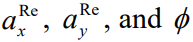determines the state of polarization. We can rewrite the Plane-Wave equation in linear algebraic notation, where

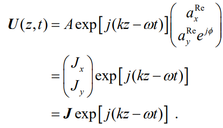
J is the Jones Vector.

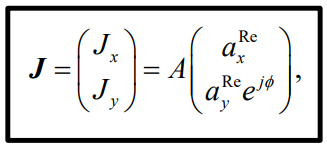
This is the notation Zemax uses for all its inputs to Polarization. Remember, phi is the difference between X-Phase and Y-Phase. The coefficient out front, in general, is a complex number. The Polarization described by the Jones Vector will not change unless the wave reflects or refracts off an optical element. Various states were reviewed in Part 1. Table 2.1 below shows the various states of polarization using Jones vectors.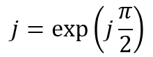

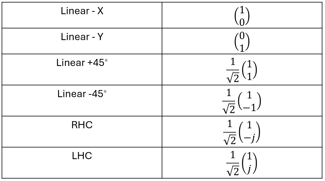
Table 2.1 Various common polarization states for input into Zemax.

Using Jones Vectors in Zemax OpticStudio

Zemax accepts Jones Matrix inputs for Polarization States; however, it does not directly output Jones Matrix data. Jones vectors are a great way to quickly review the current polarization state, and although Zemax will not output the final polarization state in this form, they can still be used to quickly evaluate the state.

For example, if we input Linear +45 degrees and pass through an ideal QWP using the Jones Matrix surface in Sequential Mode (Jones Matrix surface is similar to the Paraxial Surface, in that the Paraxial Surface creates a perfect focus, a Jones Matrix creates a perfect phase change), we should create a -pi/2 phase difference, Right Hand Circular (RHC).

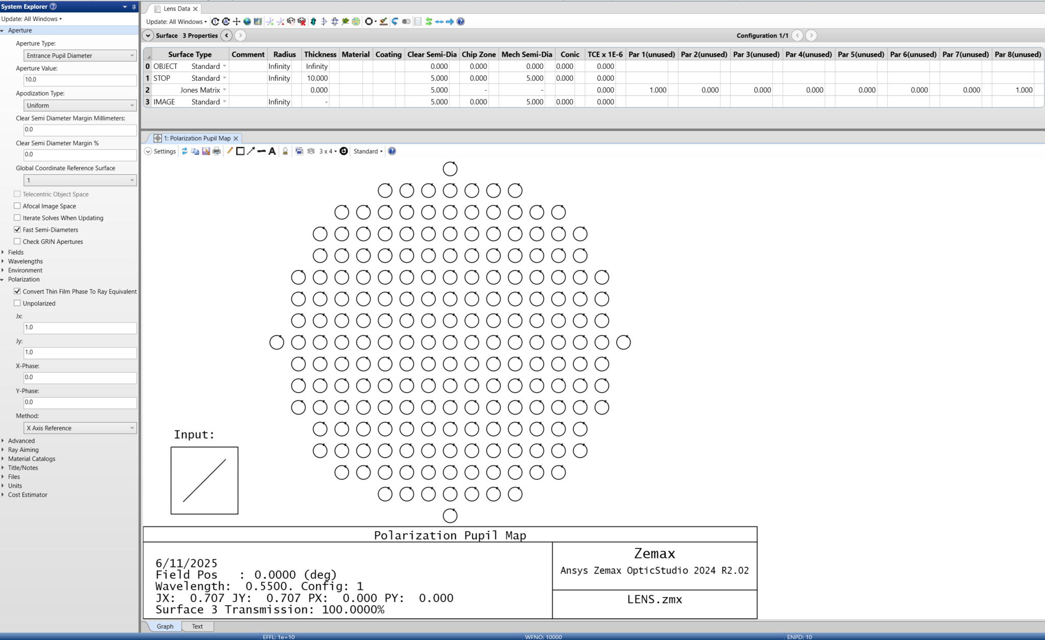
Table 2.2 Example of Linear 45-degree input through an Ideal QWP, which creates RHC.

We can confirm the state of polarization after the Jones Matrix QWP by clicking the text tab at the bottom of the Polarization Pupil Map. This is useful because the polarization state may not be easily identifiable (in this case, it is relatively obvious, but it is always good engineering to check for confirmation).

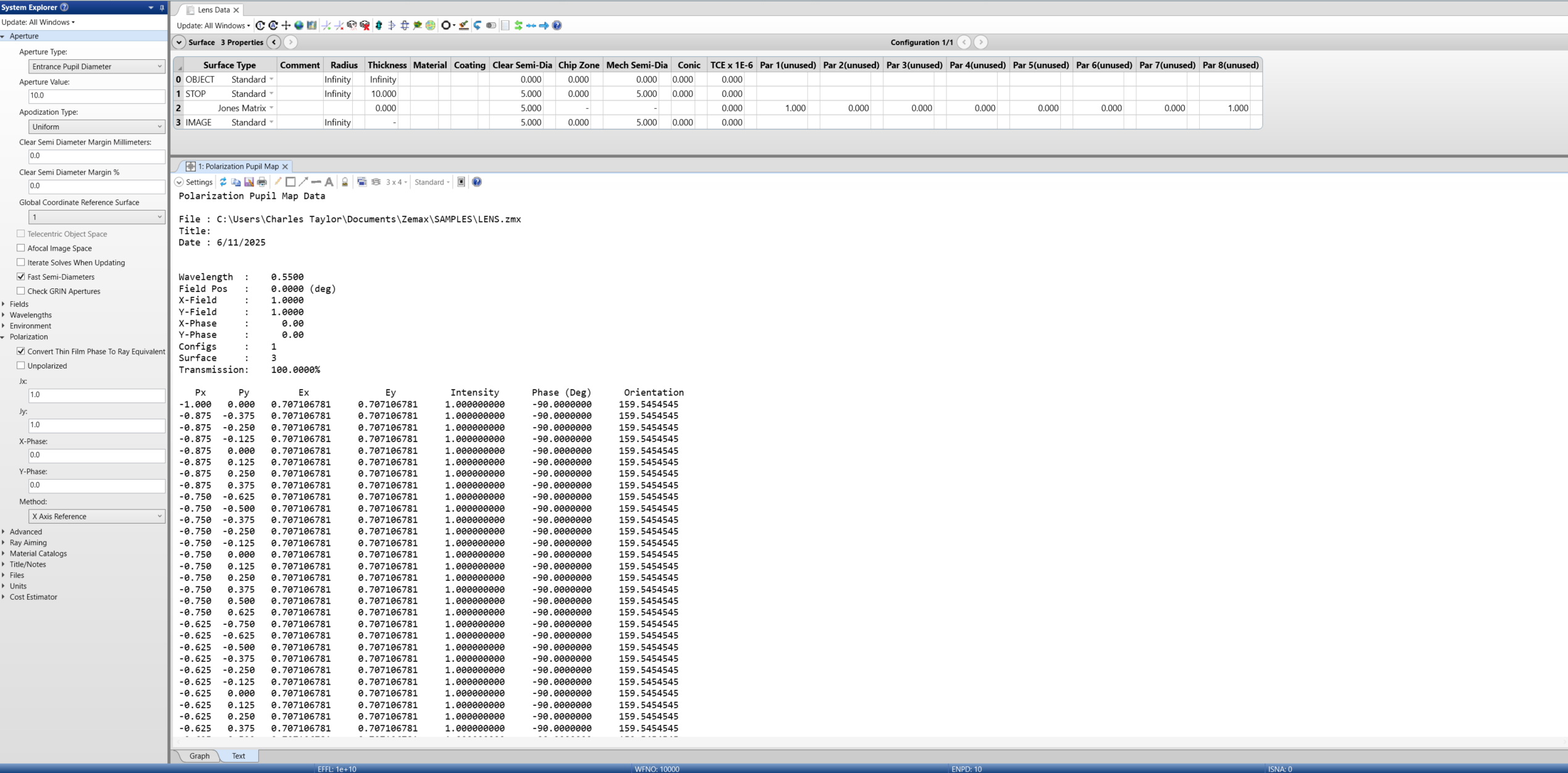
Table 2.3 Example of Linear 45 degree input through an Ideal QWP, text tab on Polarization Pupil Map.

In the text tab of the Polarization Pupil Map, each pupil position is displayed with information about the polarization state. Here, every position is the same, but that is not always the case. Px is the Pupil Coordinate along the x-axis. Py is the Pupil Coordinate along the y-axis. Ex is the magnitude of the Electric Field, and the 1st row of the Jones vector. Ey is the magnitude of the Electric Field, and the 2nd row of the Jones vector. Intensity is normalized. Intensity or transmission. Phase (Deg) is the phase difference between Phase X and Phase Y. Orientation is the major axis of the polarization ellipse in degrees, typically measured from the x-axis.

We can plug in the values like so,

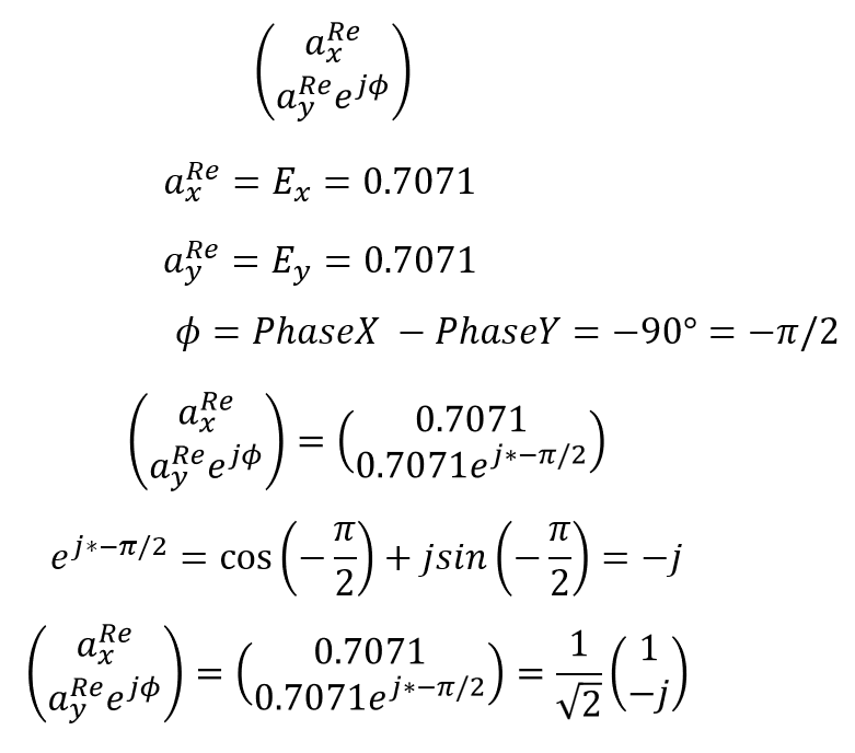
and show that this is indeed Right-Hand Circular Polarization. This information can also be gathered from the Polarization Ray Trace, which is extremely useful when dealing with complex polarization components and states. This is because we can call the POLTRACE from a Macro and compile this information into a Jones Matrix. The Macro code for this is below, but the details of this Macro are out of scope for this blog post.

ZPL Macro: Extracting Jones Vector Data from Polarization Ray Trace

————————————————————————————————————

! This macro is intended to compute Polarization as a Jones Vector from Polarization Ray Tracing.

! define the ray to be traced.
hx = 0
hy = 1
px = 0
py = 0
wavelength = PWAV()
last_surface=NSUR()

FORMAT 4.3
PRINT “Trace this ray: ”
PRINT “hx = “, hx
PRINT “hy = “, hy
PRINT “px = “, px
PRINT “py = “, py

GOSUB get_trans
trans_config_1 = intensity_1
electric_real_x = Ex_real
electric_real_y = Ey_real
electric_real_z = Ez_real
electric_imag_x = Ex_imag
electric_imag_y = Ey_imag
electric_imag_z = Ez_imag
A_x_1 = SQRT(Ex_real*Ex_real + Ex_imag*Ex_imag)
A_y_1 = SQRT(Ey_real*Ey_real + Ey_imag*Ey_imag)
A_z_1 = SQRT(Ez_real*Ez_real + Ez_imag*Ez_imag)
Phase_x_1 = Phase_X_1
Phase_y_1 = Phase_Y_1
Phase_z_1 = Phase_Z_1
EMajor = SQRT(0.5*(A_x_1*A_x_1 + A_y_1*A_y_1 + SQRT((A_x_1*A_x_1*A_x_1*A_x_1) + (A_y_1*A_y_1*A_y_1*A_y_1) + 2*(A_x_1*A_x_1*A_y_1*A_y_1)*COSI(2*(Phase_x_1 – Phase_y_1)))))
Eminor = SQRT(0.5*(A_x_1*A_x_1 + A_y_1*A_y_1 – SQRT((A_x_1*A_x_1*A_x_1*A_x_1) + (A_y_1*A_y_1*A_y_1*A_y_1) + 2*(A_x_1*A_x_1*A_y_1*A_y_1)*COSI(2*(Phase_x_1 – Phase_y_1)))))
Epsilon = 0.0000000000001
Ap = (180/3.1415926535)*(1/2)*ATAN((2*A_x_1*A_y_1*COSI(Phase_x_1 – Phase_y_1)) / (A_x_1*A_x_1 – A_y_1*A_y_1 + Epsilon))

PRINT “Jones Vector Data Config 1”
PRINT “A_x = “, A_x_1
PRINT “A_y = “, A_y_1

PRINT “Phase_x [deg] = “, Phase_x_1*(180/3.1415926535)
PRINT “Phase_y [deg] = “, Phase_y_1*(180/3.1415926535)
PRINT “Phase_diff [deg] = “, Phase_x_1*(180/3.1415926535) – Phase_y_1*(180/3.1415926535)
PRINT “Major Axis Length = “, EMajor
PRINT “Minor Axis Length = “, Eminor
PRINT “Angle between Major and x-axis [deg] = “, Ap

PRINT
PRINT “Program End”
END

SUB get_trans
POLDEFINE 0,1,150,60
SETCONFIG 1
intensity_1 = 0

POLTRACE hx, hy, px, py, wavelength, 1, last_surface
!GOSUB print_vector
Ex_real = VEC1(2)
Ey_real = VEC1(3)
Ez_real = VEC1(4)
Ex_imag = VEC1(5)
Ey_imag = VEC1(6)
Ez_imag = VEC1(7)
Phase_X_1 = VEC1(16)
Phase_Y_1 = VEC1(17)
Phase_Z_1 = VEC1(18)

intensity_1 = (Ex_real*Ex_real) + (Ey_real*Ey_real) + (Ez_real*Ez_real)
intensity_1 = intensity_1 + (Ex_imag*Ex_imag) + (Ey_imag*Ey_imag) + (Ez_imag*Ez_imag)

RETURN

SUB print_vector
FORMAT 1.0
PRINT “Electric Field Data from each configuration”
FORMAT 4.6
PRINT “Ex_real_1 = “, VEC1(2)
PRINT “Ey_real_1 = “, VEC1(3)
PRINT “Ez_real_1 = “, VEC1(4)
PRINT “Ex_imag_1 = “, VEC1(5)
PRINT “Ey_imag_1 = “, VEC1(6)
PRINT “Ez_imag_1 = “, VEC1(7)

PRINT
RETURN

————————————————————————————————————

Jones Matrices for Optical Elements

In Jones Calculus, optical elements are assumed to be linear. Each element is a 2×2 Matrix, M, that operates on an input Jones vector to output a new Jones vector as shown mathematically below.

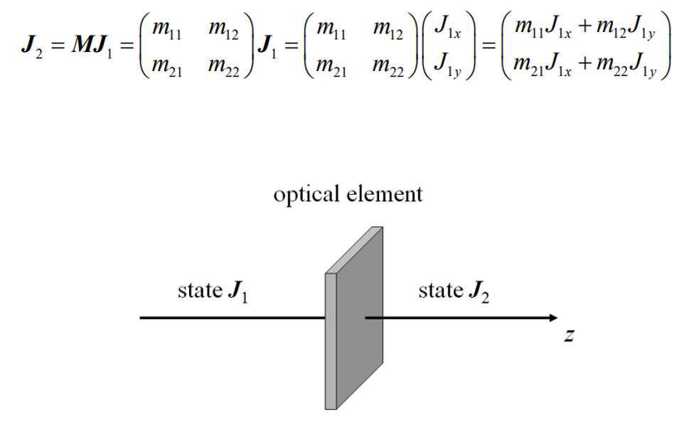
Figure 2.4 Jones vector 1 mathematically operated on by the optical element to output Jones Vector 2.

Multiple elements are computed as follows.

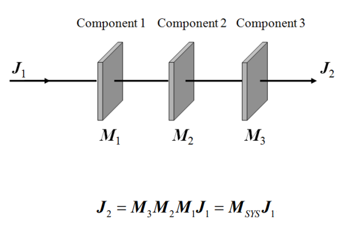
Figure 2.5 Jones Vector mathematical operation for multiple elements.

Jones Matrices for Mirrors: Reflection and Transmission

For a Mirror, the corresponding Jones matrix describing reflection is,

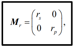
and the transmitted Jones matrix is

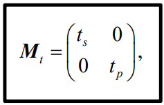
and the coefficients rs and rp are Fresnel reflection coefficients for s- and p-polarizations, respectively, while ts and tp are Fresnel transmission coefficients for s- and p-polarizations, respectively. The reflection and transmission coefficients are derived from matching boundary conditions at the interface. They are given here for context, but not derived.

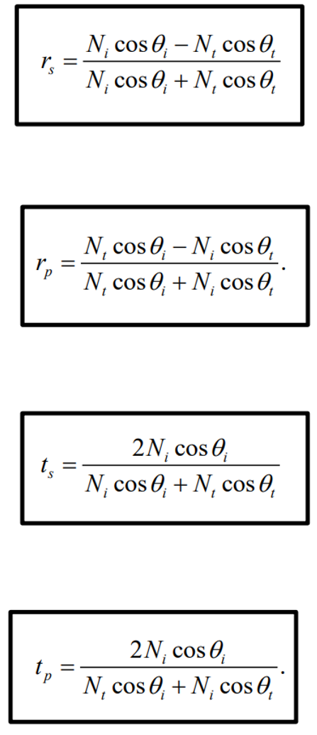
The thetas are derived from Snell’s Law.

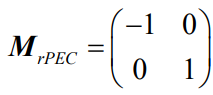
A perfect electrical conductor is called the mirror matrix, as shown below.

Not all interfaces will produce a perfect reflection, and most real-life mirrors will induce a phase shift that changes the polarization state. It is important to collect as much coating and substrate information as possible from vendors to properly simulate the optical component in Zemax. For example, the mirror matrix for an aluminum mirror looks like,

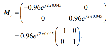
which will induce a Phase shift and change the polarization state.

Example: RHC Polarization on an Aluminum Mirror

If a RHC polarization is incident on an ALUM MATE from the coating file using the coating FP, we can see that just before the mirror, the state is RHC, and right after it is elliptical.

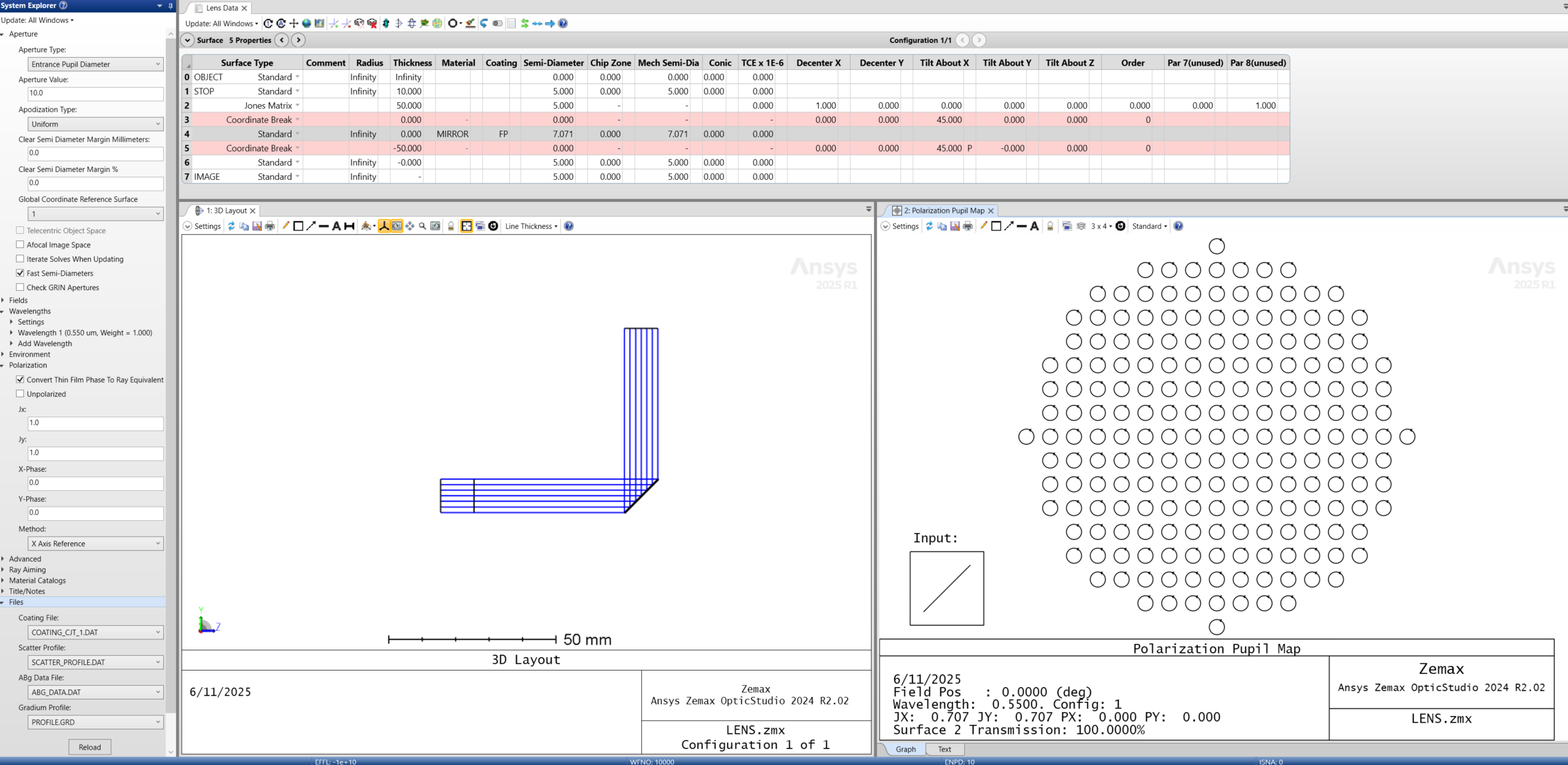
Figure 2.6 RHC Polarization just before the Aluminum Mirror.

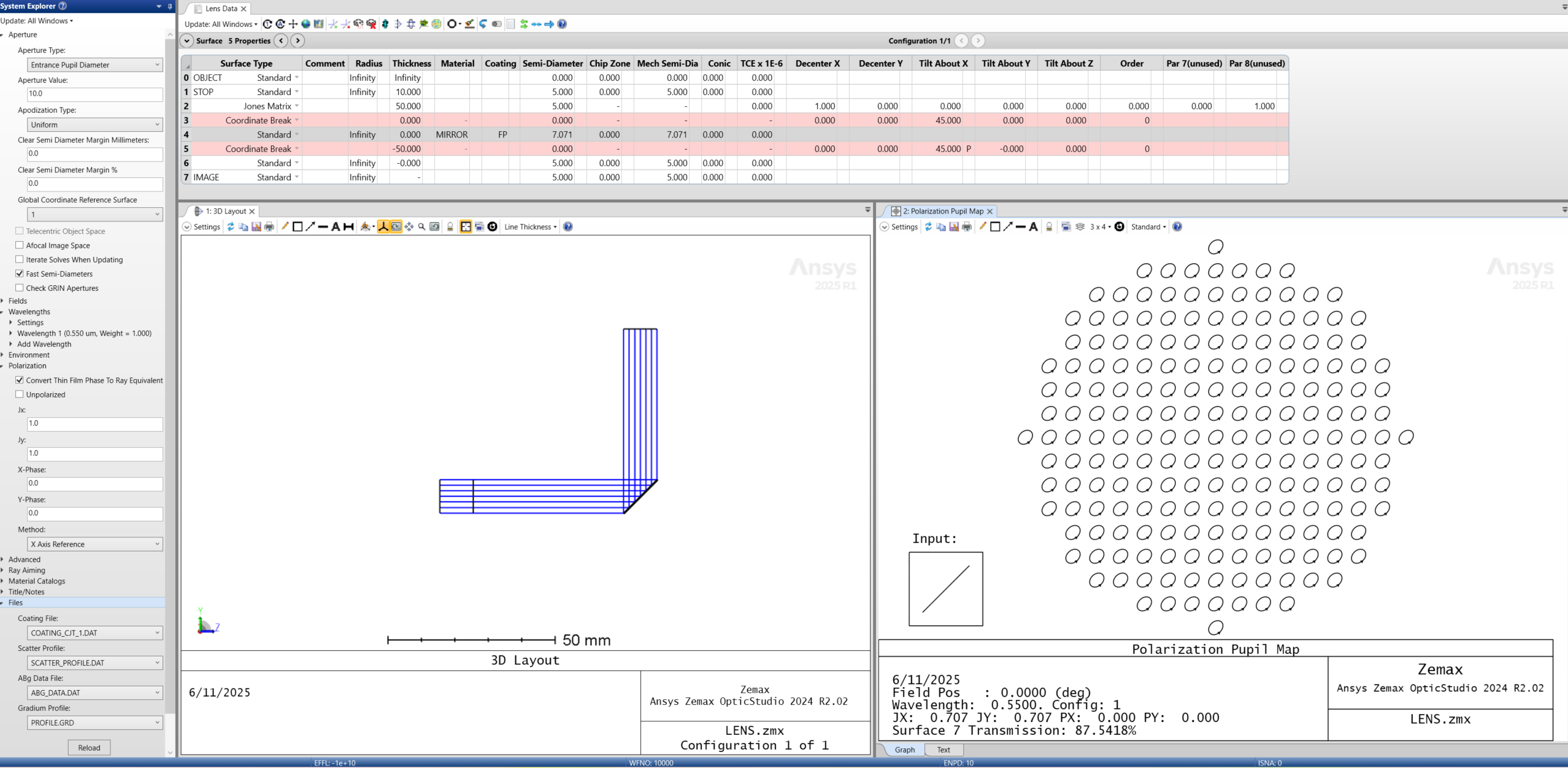
Figure 2.7 RHC incident on Aluminum Mirror and acquired a Phase shift. After the Mirror, the polarization state is elliptical.

Use the Macro from above, and we can see what the parameters of this new polarization state are after the Aluminum Mirror.

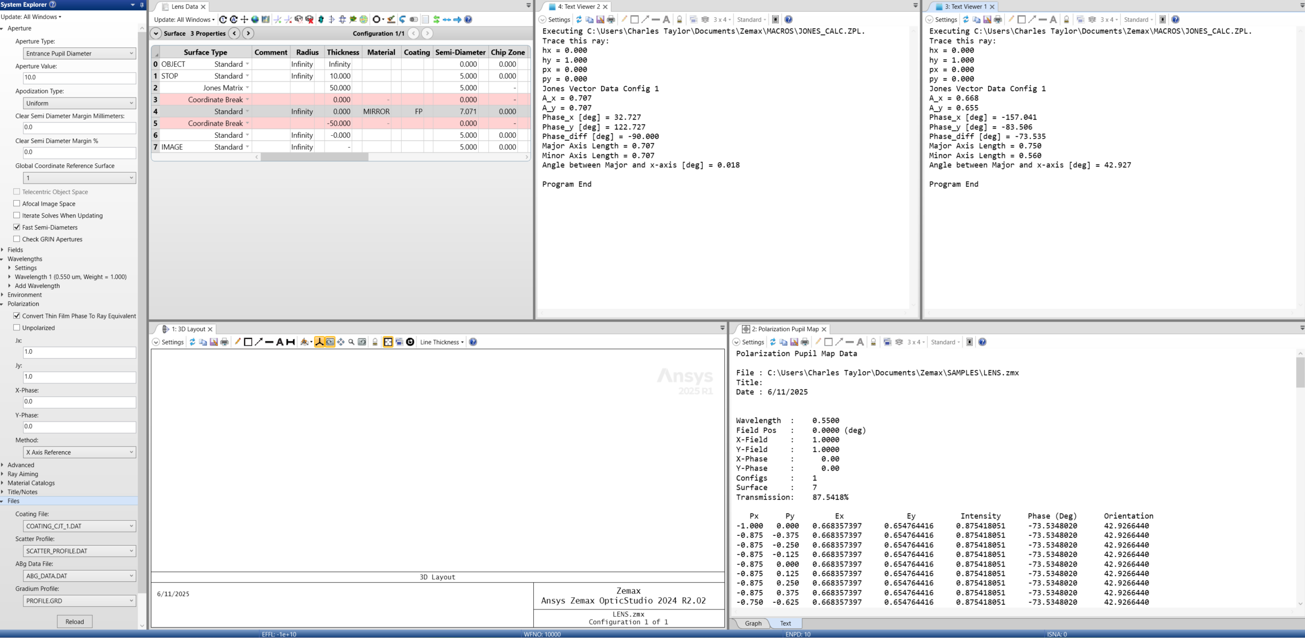
Figure 2.8 Jones Calc Macro before (Top middle) and after Mirror (Top right).

Image and notation credit to Prof. Tom D. Milster, University of Arizona

Applying Jones Calculus for Polarization Modeling in Zemax

Jones notation is widely used in Zemax OpticStudio as discussed in the first part. Jones Matrices also allow for the correct modeling of various polarization components that would otherwise be difficult to understand. This framework makes it easier to model and optimize these optical components.

Want to go deeper with polarization modeling in Zemax? SimuTech Group’s Zemax 101 training course covers optical design fundamentals, including aberrations and wave optics. For more on Zemax’s full capabilities, read our guide to maximizing optical workflows with Ansys Zemax. Contact us to discuss your optical simulation needs.