
 Contact Us
Introduction to Silicon Optical Properties
Optical design depends on material response, not only on geometry. Refractive index controls phase and confinement; extinction coefficient and absorption determine loss; and the dielectric response connects electronic structure to the interaction of a material with light. QuantumATK provides a practical environment for calculating these quantities from an atomistic model, allowing engineers to investigate how material composition and electronic structure influence device-relevant optical behavior.
This article extends the validated bulk-silicon workflow from the Atomic Structure to Device-Relevant Parameters blog. It uses an optimized silicon structure and a converged electronic calculation as the foundation for an optical-spectrum analysis. The goal is to demonstrate a reproducible QuantumATK workflow, explain how its outputs support engineering decisions, and show how simulation settings and physical approximations should be documented when results are compared with published measurements.
It uses an optimized silicon structure and a converged electronic calculation as the foundation for an optical-spectrum analysis. The focus is on interpreting quantities that photonics and semiconductor engineers can use, while keeping the limits of an independent-particle DFT spectrum explicit.
Why Optical Response Follows Band Structure
Band structure identifies allowed electronic states. Optical response adds transition probabilities: it asks which occupied-to-unoccupied transitions couple to light at each photon energy. The imaginary part of the dielectric function captures absorption-related interband transitions; the real part is connected to dispersion through the Kramers-Kronig relation.
For cubic silicon, the macroscopic optical response should be nearly isotropic in equivalent crystallographic directions. That makes silicon a useful validation material before studying anisotropic crystals, strained films, interfaces, or photonic materials.
The article answers four questions:
- What optical quantities can be extracted from the complex dielectric response?
- How do dielectric function, refractive index, extinction coefficient, reflectivity, and absorption relate?
- Which calculation settings control the resolution and credibility of the spectrum?
- What can—and cannot—be concluded from an independent-particle optical calculation?
QuantumATK Workflow
The calculation reused the HSE06-optimized bulk-silicon geometry from Blog 1 and attached an LCAO TB09-LDA calculator for the optical electronic structure. QuantumATK OpticalSpectrum was then evaluated with the Kubo-Greenwood formalism to obtain the complex dielectric response and derive refractive index, extinction coefficient, absorption coefficient, and reflectivity [1-3]. This structure-to-property workflow keeps the atomic model, electronic method, convergence settings, analysis objects, and exported results connected in one reproducible simulation process.
- Start from the optimized bulk silicon configuration established in Blog 1.
- Choose an electronic-structure method and basis appropriate to the optical energy range, material, and accuracy goal.
- Converge the optical k-point grid separately from the self-consistent k-point grid.
- Set an energy window that covers the transitions you plan to discuss.
- Choose and document spectral broadening and the number of valence and conduction bands.
- Calculate OpticalSpectrum, then export the complex dielectric function and derived optical constants.
Table 1. Settings to record for a reproducible silicon optical-spectrum calculation
| Setting | Value used in this study |
| Starting configuration | Optimized crystalline diamond-cubic Si; HSE06 lattice constant a = 5.455180 Å |
| Electronic-structure method | LCAO TB09-LDA; LDA DoubleZetaDoublePolarized basis |
| SCF k-point grid | 9 x 9 x 9 |
| Optical k-point grid | 15 x 15 x 15; checked against 18 x 18 x 18 |
| Energy range and spacing | 0.00-6.00 eV; 0.01 eV spacing |
| Broadening | 0.10 eV |
| Valence/conduction bands | 4 valence / 8 conduction; checked against 12 conduction |
| Transition operator | VelocityOperator; Full method |
1. Understanding Silicon Optical Properties Through Dielectric Response
The complex dielectric function is commonly written as ε(ω) = ε₁(ω) + iε₂(ω). The imaginary component ε₂ is associated with allowed optical transitions. The real component ε₁ determines dispersion and, together with ε₂, yields refractive index and extinction coefficient.
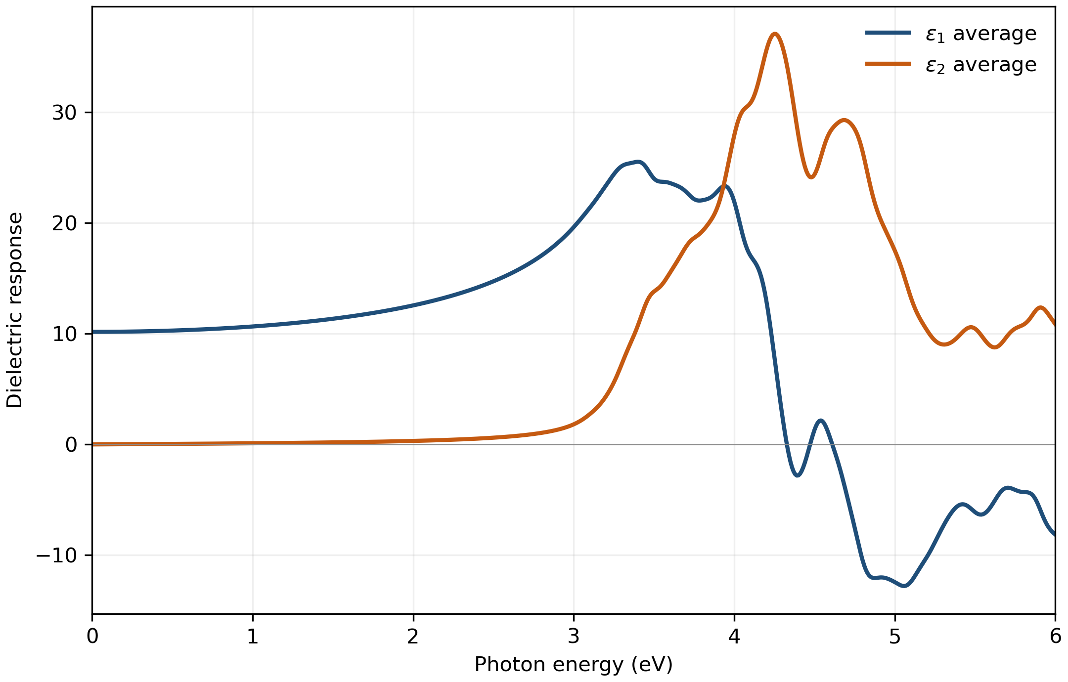
The calculated electronic dielectric response is ε₁(0) = 10.1626. The imaginary component rises gradually through the broadened low-energy tail and develops its largest peak, ε₂ ≈ 37.1, at approximately 4.25 eV. The peak energy lies in the region of the strong high-energy interband structure observed experimentally in crystalline silicon near 4.3 eV [4], while its exact amplitude remains more sensitive to optical k-point sampling. The weak sub-gap tail and any threshold extracted from it are controlled by the imposed 0.10 eV broadening and must not be identified with silicon’s experimental phonon-assisted indirect absorption edge.
Comparison with published silicon data provides context for interpreting this specific calculation. The present workflow gives electronic ε₁(0) = 10.1626 and n(0.80 eV) = 3.2352, compared with published values of approximately 11.7-11.9 and 3.48, respectively [1,5,6]. The calculation captures the expected order and overall optical behavior, while the numerical differences depend on the selected TB09-LDA independent-particle model, basis, and calculation settings. QuantumATK enables users to vary and converge these choices to balance accuracy and computational cost for a particular application. This comparison illustrates the distinction between numerical convergence, which establishes stability for a chosen setup, and physical validation, which evaluates how well that setup represents the intended material and operating conditions.
For cubic silicon the three diagonal tensor components are numerically identical: the maximum epsilon1 difference among xx, yy, and zz over the sampled energy range was 2.13 × 10⁻¹⁴. This confirms that the calculation preserves the expected cubic isotropy.
2. From Dielectric Response to Refractive Index and Absorption
The complex refractive index is N(ω) = n(ω) + ik(ω). Here n is the refractive index and k is the extinction coefficient. The absorption coefficient is α(ω) = 2ωk/c. These silicon optical properties are derived from the same complex dielectric response, so they should be interpreted together rather than as unrelated curves.
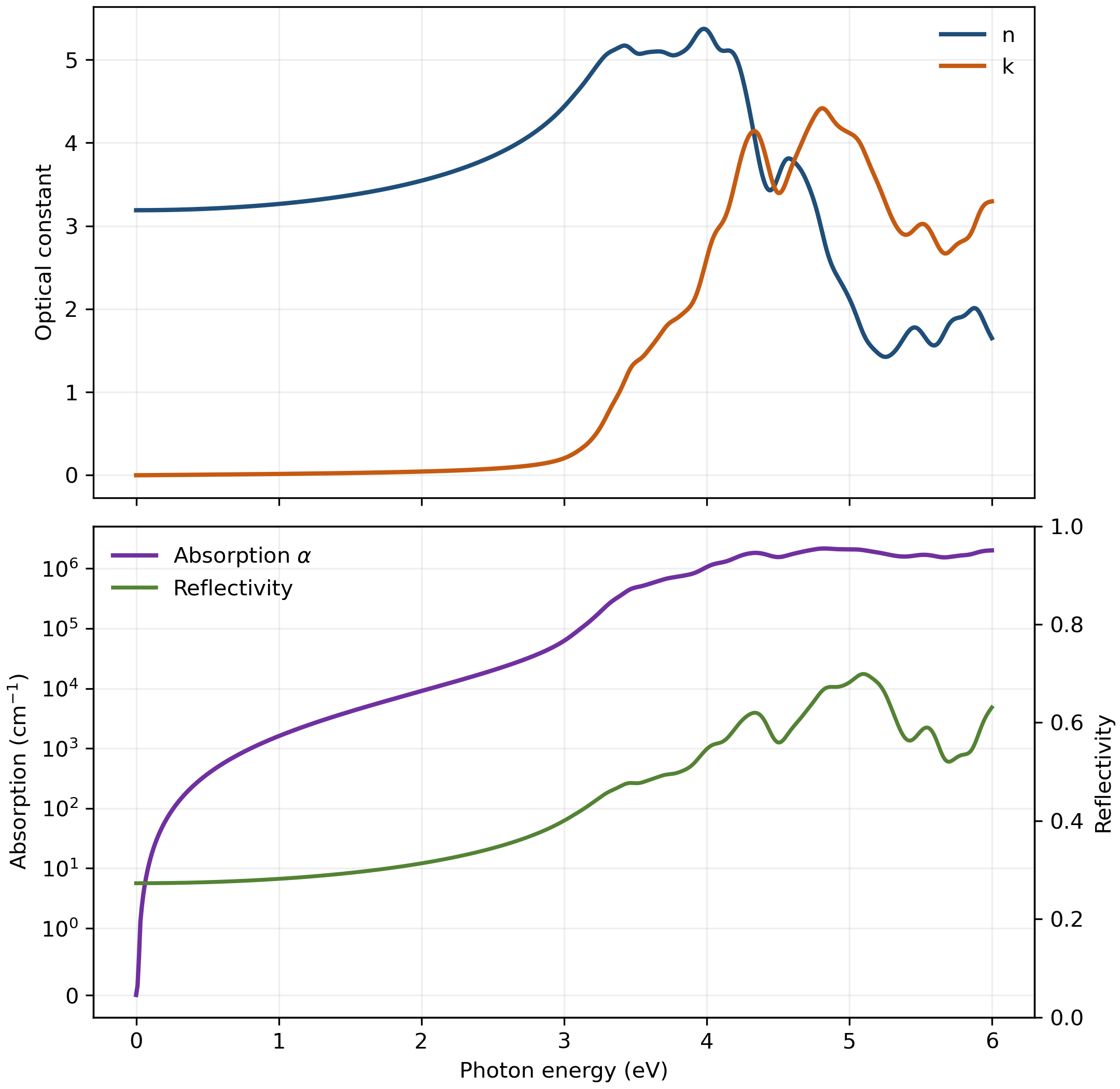
At 0.80 eV (approximately 1550 nm), the broadened independent-particle calculation gives n = 3.2352, k = 0.01222, reflectivity R = 0.2785, and absorption α = 9.91 × 10² cm⁻¹. At this sub-gap energy, the calculated k and α are dominated by the imposed 0.10 eV spectral broadening and should not be interpreted as predictions of the physical telecom-wavelength absorption of crystalline silicon. Experimental studies of high-resistivity crystalline silicon report much lower absorption near 1550 nm, with values that depend on sample properties and measurement conditions [7,8]. The calculated values are therefore reported here only to illustrate the low-energy tail of this broadened spectrum. Likewise, the first point at which α reaches 10³ cm⁻¹, 0.81 eV, is an operational threshold of the calculation rather than the experimental indirect absorption edge. Within the plotted range, the maximum absorption is 2.16 × 10⁶ cm⁻¹ at 4.82 eV.
What the Spectrum Does and Does Not Mean
A direct electronic transition energy is not, by itself, an absorption spectrum. Optical intensity depends on transition matrix elements and the k-resolved joint density of states. The OpticalSpectrum setup used here describes vertical electronic transitions within an independent-particle treatment and applies a selected numerical broadening [2]. It does not explicitly represent electron-hole interactions, phonon-assisted indirect absorption, or temperature-dependent band renormalization. The 0.10 eV broadening smooths the spectrum for analysis, but it also produces a low-energy tail that is a feature of this numerical representation rather than an additional physical absorption mechanism. These boundaries define the scope of the chosen calculation and help engineers decide whether it is sufficient for the application or should be supplemented with additional physics, calibrated material data, or experimental validation.
Results Summary
Table 2 reports values exported from the final OpticalSpectrum. Because bulk silicon is cubic, directional averages are reported; the diagonal tensor components were identical within numerical precision.
Table 2. Optical quantities to report from the silicon workflow
| Quantity | Calculated result | Engineering interpretation |
| Zero-frequency electronic dielectric response | Electronic ε₁(0) = 10.1626 (directional average) | Screening and material dispersion |
| Refractive index at selected photon energy | n(0.80 eV) = 3.2352 | Phase velocity and optical confinement |
| Extinction coefficient at selected photon energy | k(0.80 eV) = 0.01222 | Low-energy behavior of this broadened spectrum; not a prediction of intrinsic telecom-wavelength loss |
| Operational absorption threshold / main feature | Operational α >= 10³ cm⁻¹ at 0.81 eV; ε₂ peak at 4.25 eV | Method-specific transition scale; the 0.81 eV threshold is not the experimental indirect absorption edge |
| Peak absorption coefficient | 2.16 × 10⁶ cm⁻¹ at 4.82 eV | Optical-loss magnitude within calculated model |
| Reflectivity at selected photon energy | R(0.80 eV) = 0.2785 | Interface reflection and optical coupling |
Engineering Value of the Completed QuantumATK Workflow
The completed QuantumATK workflow for calculating silicon optical properties provides more than a single plot: it contains the ground-state configuration, convergence spectra, final OpticalSpectrum object, exported numerical data, and publication figures. This traceability helps engineering teams review assumptions, repeat calculations, compare material options, and update the model as project requirements evolve.
- The HSE06-optimized bulk-silicon configuration from Blog 1 was reused, with lattice constant a = 5.455180 Å.
- For optical properties, the structure was assigned an LCAO TB09-LDA calculator with the LDA DoubleZetaDoublePolarized basis, a 9 x 9 x 9 SCF grid, 125 Ha density mesh cutoff, and 300 K occupation broadening.
- The final OpticalSpectrum covers 0-6 eV with 0.01 eV spacing, 0.10 eV spectral broadening, four valence bands, eight conduction bands, a 15 x 15 x 15 optical grid, the Full method, and the VelocityOperator. No intraband Drude term was included for intrinsic bulk silicon.
- Optical-grid convergence was checked at 9, 12, 15, and 18 points per reciprocal direction. From 15 to 18, ε₁(0) changed by 0.036%, n(0.80 eV) by 0.019%, and the principal ε₂ peak position by 0.02 eV. The peak height changed by about 6.4%, so absolute peak amplitudes remain more grid sensitive than the low-energy dielectric quantities.
- The unoccupied-band window was checked with 4, 8, and 12 conduction bands at the 15 x 15 x 15 optical grid. Increasing from 8 to 12 changed ε₁(0) by 0.078% and n(0.80 eV) by 0.038%, while the main ε₂ peak height was unchanged to better than 0.001%.
Silicon Optical Properties Conclusion
This silicon example shows the value of QuantumATK as an engineering learning and decision-support platform: it links atomistic structure, electronic behavior, optical response, convergence testing, and exportable results in a single workflow. The most useful outcome is not an isolated number, but a transparent model that helps teams understand material behavior, evaluate alternatives, communicate confidence and limitations, and decide what additional simulation or measurement is appropriate for the application.
Continue the QuantumATK Series: Explore how electronic structure translates into semiconductor device behavior in our next article, Silicon P-N Junction Simulation with NEGF in QuantumATK, examining band bending, electron transmission, and current flow under applied bias.
Need help with semiconductor materials modeling in QuantumATK?
SimuTech Group can help your team use Synopsys QuantumATK to evaluate electronic structure, band gaps, density of states, effective mass, and other atomistic material properties that support semiconductor and device-level modeling.
- Synopsys QuantumATK Y-2026.03 Documentation, “Optical Properties of Silicon.” https://docs.quantumatk.com/tutorials/optical/optical.html
- Synopsys QuantumATK Y-2026.03 Documentation, “OpticalSpectrum.” https://docs.quantumatk.com/manual/Types/OpticalSpectrum/OpticalSpectrum.html
- Synopsys QuantumATK Y-2026.03 Documentation, “Optical Property Calculations.” https://docs.quantumatk.com/intro/intro_tutorials/optical-properties-SiO2/optical-properties-SiO2.html
- H. R. Philipp and E. A. Taft, “Optical Constants of Silicon in the Region 1 to 10 eV,” Physical Review 120, 37-38 (1960). https://doi.org/10.1103/PhysRev.120.37
- W. C. Dunlap, Jr. and R. L. Watters, “Direct Measurement of the Dielectric Constants of Silicon and Germanium,” Physical Review 92, 1396-1397 (1953). https://doi.org/10.1103/PhysRev.92.1396
- H. H. Li, “Refractive Index of Silicon and Germanium and Its Wavelength and Temperature Derivatives,” Journal of Physical and Chemical Reference Data 9, 561-658 (1980). https://doi.org/10.1063/1.555624
- J. Degallaix et al., “Bulk Optical Absorption of High Resistivity Silicon at 1550 nm,” Optics Letters 38, 2047-2049 (2013). https://doi.org/10.1364/OL.38.002047
- J. Steinlechner et al., “Optical Absorption Measurements on Crystalline Silicon Test Masses at 1550 nm,” Classical and Quantum Gravity 30, 095007 (2013). https://doi.org/10.1088/0264-9381/30/9/095007

Majid Ebnali Heidari, PhD
Engineering Manager – Optics/Photonics, SimuTech Group
Majid Ebnali Heidari, Ph.D., is an Engineering Manager at SimuTech Group with 18+ years of experience in photonics, optics, electronics, EDA simulation, academia, and industry. He specializes in multiscale optics and photonics simulation, optoelectronic device modeling, optical system validation, and technical training. His expertise spans nanoscale photonic structures, micro-scale optoelectronic devices, and system-level optical workflows using Ansys Lumerical, Zemax OpticStudio, Speos, and multiphysics simulation tools. He helps engineering teams apply advanced simulation to real-world product development, design validation, and engineering decision-making.