
 Contact Us
Introduction to Silicon p-n Junction Simulation
Silicon p-n junction simulation helps engineers understand how electronic structure, electrostatic potential, and charge transport interact within semiconductor devices. While bulk-silicon calculations characterize material properties, modeling a p-n junction introduces contacts, doping profiles, and applied voltage to examine device behavior under equilibrium and finite-bias conditions.
Synopsys QuantumATK uses the non-equilibrium Green’s function (NEGF) formalism to model electron transport through open, two-terminal systems. By connecting a silicon crystal to left and right electrodes, engineers can investigate band bending, transmission, and current flow at the atomistic level.
Building on our previous articles covering bulk-silicon electronic structure and optical properties, this tutorial examines a reproducible p-n junction workflow, including device construction, numerical convergence, and forward- and reverse-bias analysis. It also highlights the physical assumptions and limitations that must be considered when interpreting simulation results.
What the Reader Will Learn
- How a periodic silicon crystal becomes a two-probe device with left and right electrodes.
- Why the central region must be long enough for the electrostatic potential to become bulk-like near both electrodes.
- How Hartree difference potential, projected local density of states (PLDOS), and transmission reveal different parts of the same junction physics.
- How the NEGF/Landauer framework connects transmission inside the bias window to electrical current.
- Which results are physical insights and which are consequences of the idealized model used in this study.
1. From Bulk Silicon to P-N Junction Simulation
Bulk calculations use periodic boundary conditions and describe an effectively infinite crystal. A transport device has a different mathematical structure: a finite central region is connected to semi-infinite electrodes that inject and absorb carriers. QuantumATK treats this open system with the non-equilibrium Green’s function (NEGF) formalism [1,2].
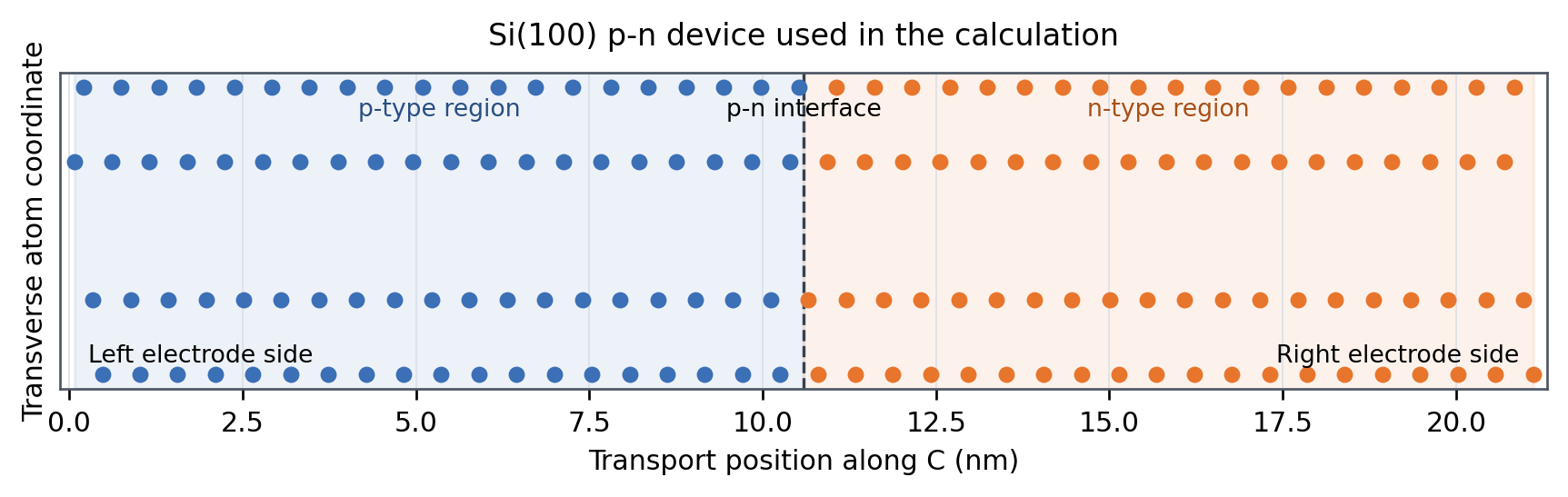
The device is divided into left electrode, central region, and right electrode. The outer portions of the central region must reproduce the electrostatic environment of their adjacent electrodes. If the potential has not flattened before the boundaries, the screening approximation is not satisfied and the calculated junction can be contaminated by its finite length.
Device Construction Used for the Study
- Start from the optimized crystalline-silicon structure established in Blog 1 (a = 5.455180 Å). QuantumATK may display this database entry as ‘Silicon (alpha)’; here, crystalline silicon is used to avoid confusing it with amorphous silicon.
- Cleave the crystal along the Si(100) direction and retain the 1 x 1 surface unit cell.
- Use 78 layers for the central region, giving a device length of approximately 20 nm.
- Create a two-probe device with the transport direction along C and retain the minimal electrode and electrode-extension lengths appropriate for the nearest-neighbor Bassani model [3].
- Apply p-type background doping of 2 x 10^19 cm^-3 to the left half and n-type background doping of 2 x 10^19 cm^-3 to the right half.
2. Numerical Model and Convergence Controls
For this first device article, a self-consistent semi-empirical tight-binding calculation provides a practical balance of physics and cost. The Bassani parameterization is available for silicon and makes a roughly 20 nm NEGF device tractable. This is a model choice, not a claim that semi-empirical NEGF replaces DFT-NEGF: chemically complex interfaces, defect states, or materials without a validated parameterization may require a first-principles Hamiltonian.
| Model component | Production setting | Why it matters |
| Hamiltonian | Semi-empirical Slater-Koster; Bassani.Si | Efficient silicon electronic structure for the long device |
| SCF convergence strategy | Direct restart for -1 V; +0.25 V staged ramp to +1 V | Stabilizes the finite-bias density and avoids direct-jump oscillation |
| Device k-point density | 4 Å x 4 Å x 150 Å; approximately 7 x 7 x 174 | Dense electrode sampling along transport; transverse Brillouin-zone integration |
| Poisson solver | FFT2D | Periodic in A/B; open Dirichlet boundaries along transport C |
| Electrode temperature | 300 K | Sets Fermi-Dirac occupations in the contacts |
| PLDOS and transmission energies | −2.0 to +2.0 eV; 401 points | Resolves band edges and the bias window |
| PLDOS/transmission transverse k-grid | 12 Å × 12 Å transverse density; generated grid approximately 20 × 20 | Transport spectra are sensitive to silicon’s conduction-band valleys |
Table 1. Reproducibility snapshot for the QuantumATK Y-2026.03 calculation. The delivered scripts preserve the generated numerical settings; retain the log files with the publication archive.
The Two Convergence Checks That Matter Most
Device length. The Hartree difference potential should become flat toward both electrodes. This is a physical screening check, not merely a numerical nicety. If it does not flatten, increase the central-region length before interpreting the built-in potential or depletion width [4].
Transverse k-point sampling. PLDOS and transmission depend on the valleys near the silicon conduction-band minimum. Compare at least two transverse meshes and show that the band edges, integrated transmission, and current no longer change materially at the chosen grid.
3. Understanding P-N Junction Behavior at Equilibrium
At zero applied bias, the left and right electrode chemical potentials are equal, so the net current is zero. The absence of current does not mean the junction is electrostatically featureless. Charge redistribution across the p–n interface produces a built-in potential variation across the device, which is reflected in the spatially varying Hartree difference potential.
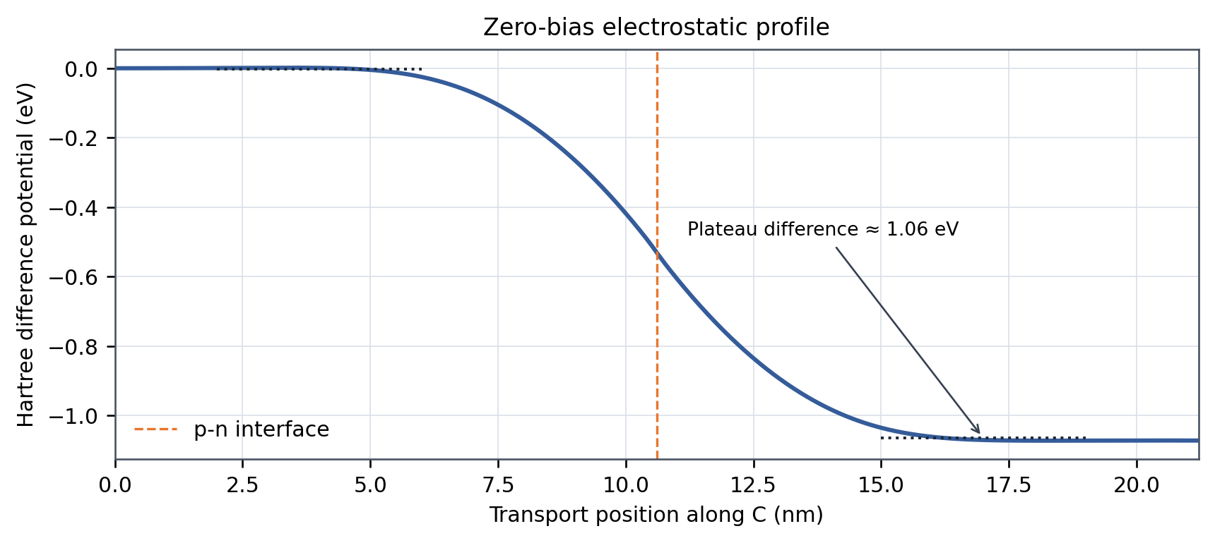
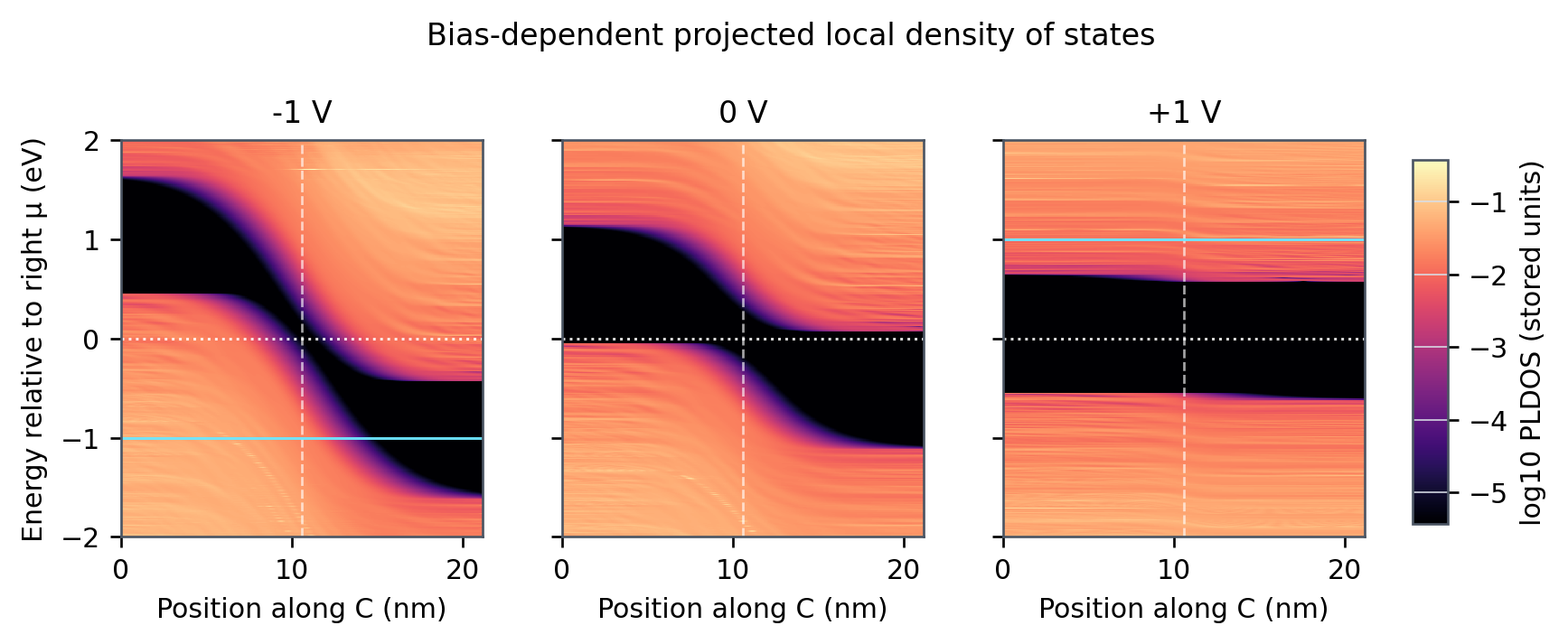
At 0 V, the Hartree difference potential is approximately bulk-like in the predefined 2–6 nm and 15–19 nm analysis windows: the standard deviations are 0.0068 and 0.010 eV, respectively. The mean values of the two plateaus differ by approximately 1.06 eV, showing the built-in junction potential variation while also indicating that the potential has become nearly flat toward both electrode sides.
PLDOS Turns Electrostatics into a Local Band Diagram
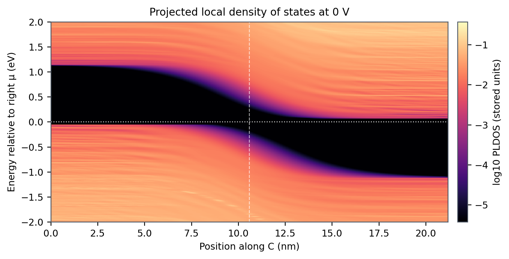
The projected local density of states maps available electronic states against both energy and position. Far from the junction, the valence-band edge should lie close to the chemical potential on the p-type side, while the conduction-band edge should lie close to it on the n-type side. Across the interface, the bending of those edges reveals the depletion width and built-in barrier.
4. Electron Transmission and the Landauer Framework
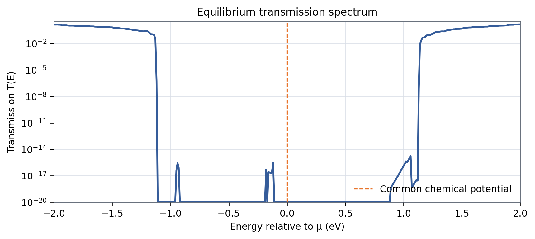
NEGF provides the energy-resolved transmission T(E) through the open device. In the equilibrium p–n junction, transmission is strongly suppressed over the energy range where propagating states through the complete device are unavailable.
The current is described by the Landauer expression:

where T(E) is the transmission function, fL(E) and fR(E) are the Fermi–Dirac occupation functions of the left and right electrodes, e is the elementary charge, and h is Planck’s constant. The factor of 2 accounts for spin degeneracy.
At equilibrium, the two electrode chemical potentials are equal, so
fL(E) = fR(E),
and the net current is zero even though finite transmission may exist at some energies.
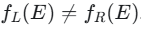
Under an applied bias, the left and right chemical potentials separate, creating an energy range in which the two contacts have different electron occupations. Transmission within this bias window can then contribute to current.
This equation also prevents a common interpretation error: a large transmission peak does not by itself imply a large current. The transmissive states must overlap an energy range where
5. Forward- and Reverse-Bias Simulation
The equilibrium calculation becomes the restart state for finite-bias simulations. In the supplied scripts, the left electrode is set to −1 V for reverse bias and +1 V for forward bias while the right electrode remains at 0 V; therefore Vbias = Vleft − Vright. Reverse bias restarts directly from 0 V. Forward bias uses smaller +0.25 V increments and restarts each point from the preceding converged state, while keeping all other model settings identical. This makes the convergence strategy explicit and follows the nearest-state restart guidance [4].
Table 2. Observed response of the completed three-point bias study.
| Bias state | Observed electrostatic response | Observed transport response |
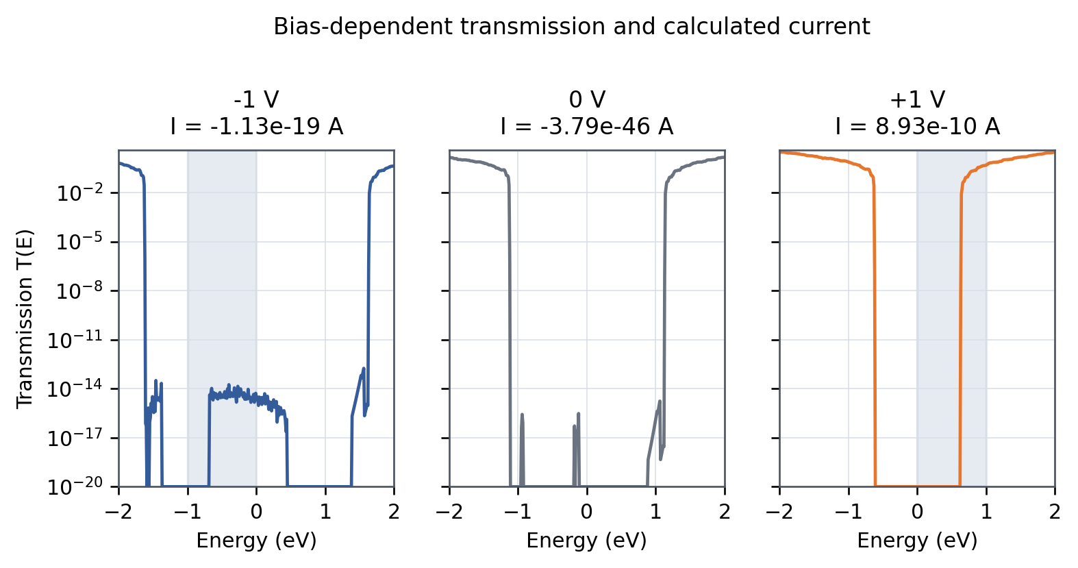
| Reverse bias (-1 V) | Mean potential difference ≈1.96 eV, but the 4 nm flatness check is not satisfied | Peak T in bias window 1.75 x 10^-14; I = -1.13 x 10^-19 A |
| Equilibrium (0 V) | Plateau difference ≈1.06 eV; flatness check satisfied | T(0) = 0; I = -3.79 x 10^-46 A (numerical zero) |
| Forward bias (+1 V) | Plateau difference ≈0.073 eV; the equilibrium electrostatic potential difference is strongly reduced | Peak T in bias window 0.467; I = 8.93 x 10^-10 A |
6. Verified Silicon P-N Junction Simulation Results
All three device calculations converged. With Vbias = Vleft – Vright and the right electrode fixed at 0 V, the calculated currents are -1.13 x 10^-19 A at -1 V, numerical zero at equilibrium, and 8.93 x 10^-10 A at +1 V. Within this ideal coherent model, the magnitude of the calculated forward current is approximately 7.9*10^9 times larger than the reverse-bias current. Because the reverse current is extremely small, this ratio should not be interpreted as a realistic device rectification ratio.
| Reported quantity | −1 V (left) | 0 V | +1 V (left) | Extraction method |
| SCF converged | Yes (25 iterations) | Yes (66 iterations) | Yes (64 iterations at +1 V; staged) | QuantumATK calculation logs |
| Current (A) | -1.13 x 10^-19 | -3.79 x 10^-46 (numerical zero) | 8.93 x 10^-10 | TransmissionSpectrum.current() |
| Electrostatic plateau difference (eV) | ≈1.96 (screening-limited) | ≈1.06 | ≈0.073 | Mean Hartree potential difference between 2-6 and 15-19 nm |
| Peak T(E) in bias window | 1.75 x 10^-14 at -0.40 eV | N/A; T(0) = 0 | 0.467 at +1.00 eV | K-point-averaged TransmissionSpectrum |
| Potential flat in 4 nm end windows | No; σL/R = 0.046/0.057 eV | Yes; σL/R = 0.0068/0.010 eV | Yes; σL/R = 0.00023/0.00046 eV | Pass criterion: both standard deviations <0.02 eV |
Table 3. Verified numerical results and physical-adequacy checks from the HDF5 files.
7. What the Silicon p-n Junction Simulation Results Mean for Semiconductor Engineering
A band structure describes which states are available in a periodic material. The completed p-n device calculation shows how those states vary spatially, how contacts populate them, and how applied voltage changes the available transmission path. At +1 V, the electrostatic plateau difference falls to approximately 0.073 eV and the peak transmission within the bias window reaches 0.467; at -1 V, the peak transmission in the bias window remains only 1.75 x 10^-14.
For engineering teams, the most transferable output is the traceable workflow rather than a single current value. QuantumATK keeps device construction, open-boundary electrostatics, restart-aware execution, HDF5 results, and spatially resolved analysis in one environment. In this study, that connected workflow exposes both the rectifying trend and a limitation: the -1 V solution converges numerically, but its potential does not satisfy the same 4 nm end-window flatness criterion used at 0 V and +1 V. The reverse-bias barrier and depletion width are therefore not reported as quantitatively validated results.
Important Limits of This Demonstration
- The structure is ideal and defect-free; interface disorder, traps, roughness, and dopant discreteness are not represented.
- The calculation demonstrates coherent elastic transport. It does not automatically include phonon-assisted transport, generation-recombination, or other inelastic leakage mechanisms.
- Background doping is a continuum-like modeling device and should not be confused with an explicit atom-by-atom dopant distribution.
- Three bias points can demonstrate rectifying behavior but do not constitute a production-quality I-V curve. Use IVCharacteristics for a denser, restart-aware voltage sweep [5].
- A semi-empirical parameter set is material-specific. New materials or chemically complex interfaces may require DFT-NEGF or a separately validated Hamiltonian.
Advancing Semiconductor Device Modeling with QuantumATK
Silicon p-n junction simulation provides a connection between electronic structure and device-level transport behavior. In this study, QuantumATK calculations demonstrated an approximately 1.06 eV equilibrium electrostatic plateau difference, negligible current at zero bias, and distinct forward- and reverse-bias transport responses within the idealized NEGF model.
By combining projected local density of states, electrostatic potential, electron transmission, and current calculations, engineers can examine how semiconductor junctions respond to applied voltage. The workflow also illustrates the importance of convergence testing, model assumptions, and physical validation when interpreting simulation results.
Extending this approach to additional bias conditions, semiconductor interfaces, and contact configurations can support further investigation of electronic device behavior and transport mechanisms.
Explore Semiconductor Device Simulation with QuantumATK
Synopsys QuantumATK provides atomistic modeling capabilities for investigating semiconductor materials, electronic structure, and electron transport. Explore how SimuTech Group can help your engineering team apply QuantumATK to materials research and semiconductor device development.
- Synopsys, QuantumATK Y-2026.03 Documentation, ‘NEGF Simulations of Electron Transport in Devices.’ https://docs.quantumatk.com/intro/intro_tutorials/electron-transport-Si-p-n/electron-transport-Si-p-n.html
- M. Brandbyge, J.-L. Mozos, P. Ordejón, J. Taylor, and K. Stokbro, ‘Density-functional method for nonequilibrium electron transport,’ Physical Review B 65, 165401 (2002). https://doi.org/10.1103/PhysRevB.65.165401
- Synopsys, QuantumATK Y-2026.03 Manual, ‘DeviceSlaterKosterCalculator.’ https://docs.quantumatk.com/manual/Types/DeviceSlaterKosterCalculator/DeviceSlaterKosterCalculator.html
- Synopsys, QuantumATK Y-2026.03 Technical Note, ‘NEGF Convergence Guide.’ https://docs.quantumatk.com/manual/technicalnotes/negf_convergence_guide/negf_convergence_guide.html
- Synopsys, QuantumATK Y-2026.03 Manual, ‘IVCharacteristics.’ https://docs.quantumatk.com/manual/Types/IVCharacteristics/IVCharacteristics.html

Majid Ebnali Heidari, PhD
Engineering Manager – Optics/Photonics, SimuTech Group
Majid Ebnali Heidari, Ph.D., is an Engineering Manager at SimuTech Group with 18+ years of experience in photonics, optics, electronics, EDA simulation, academia, and industry. He specializes in multiscale optics and photonics simulation, optoelectronic device modeling, optical system validation, and technical training. His expertise spans nanoscale photonic structures, micro-scale optoelectronic devices, and system-level optical workflows using Ansys Lumerical, Zemax OpticStudio, Speos, and multiphysics simulation tools. He helps engineering teams apply advanced simulation to real-world product development, design validation, and engineering decision-making.