Antennas play a central role in modern communication and radar systems, enabling the transmission and reception of electromagnetic signals across various platforms. Designing efficient antennas demands a deep understanding of electromagnetic principles to ensure optimal performance. This post provides an overview of the antenna simulation workflow in Ansys HFSS, a powerful design tool renowned for accurately simulating electromagnetic fields.
HFSS makes antenna design both efficient and intuitive. Its user-friendly interface and advanced features, such as parametric analysis and optimization algorithms, allow users to explore various configurations and quickly iterate designs to meet requirements.
Creating Parameterized Antenna Geometry in HFSS
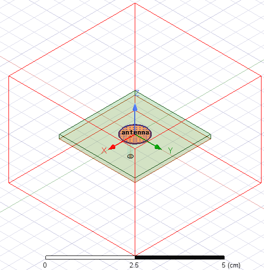
To begin, users can use the intuitive interface to draw the antenna geometry, ranging from simple structures like wire antennas to complex array configurations. One of the key advantages of HFSS is its support for parameterized geometry, which allows users to define geometric dimensions using variables rather than fixed values. This enables easy exploration of design variations and facilitates parametric studies to optimize antenna performance.
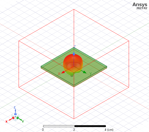
The image below shows a fully parameterized probe-fed circular patch antenna model. The Properties view below the Project Manager shows that the substrate dimensions have been parameterized. The Draw pane of the ribbon shows many 1D, 2D, and 3D drawing and Boolean operations that can be used to create model geometry.
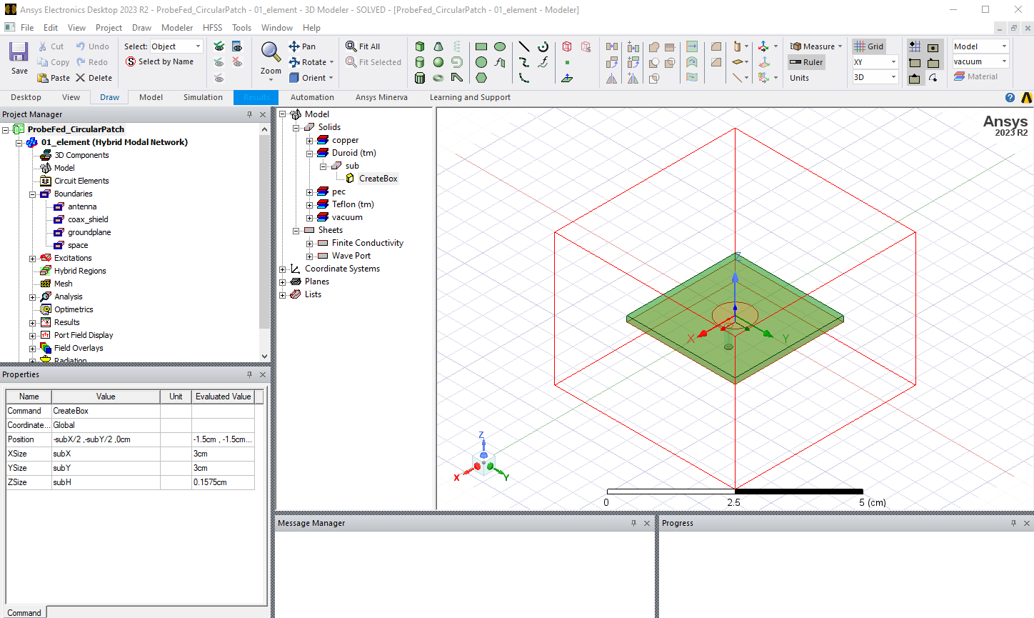
Once the geometry of the antenna element and feed structure is defined, creating an airbox around the antenna is an important step. The airbox size establishes the boundaries of the simulation domain and ensures an accurate representation of the antenna’s electromagnetic environment. In the model shown above, the airbox is defined as a region in the wireframe view.
Assigning Material Properties and Boundary Conditions
Material properties are assigned to objects within the model, including the antenna elements, PCB substrates, and surrounding structures. The material properties define how electromagnetic waves interact with the objects. The relevant material properties for antenna simulation include the dielectric permittivity, dielectric loss tangent, and electrical conductivity. By accurately specifying material properties, users can simulate antennas in realistic environments and assess their performance under different operating conditions.
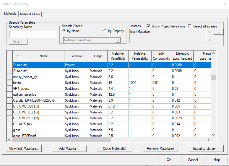
HFSS includes a materials library that contains many materials commonly used in antenna design. Users can add custom materials to the library. The material properties can be frequency-dependent, anisotropic, spatially-dependent, and/or temperature-dependent. The image below shows the materials library definition for the substrate material used in the patch antenna model.
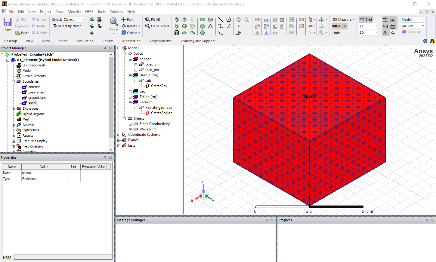
Boundary conditions play an important role in defining the behavior of electromagnetic fields at the boundaries of the simulation domain, as well as for 2D objects. For antennas, HFSS provides multiple options to specify boundary conditions that mimic an open space, allowing electromagnetic waves to propagate freely without reflections. These include second-order absorbing boundary conditions (ABC), perfectly matched layers (PML), and finite element boundary integral (FE-BI) terminations. The image below shows an absorbing boundary condition assigned to the outer faces of the airbox region.
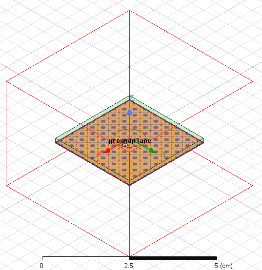
For 2D electrically conductive objects such as antennas and ground planes, a finite conductivity boundary condition is applied. HFSS includes multiple surface roughness models that can be applied to these boundaries to closely match the properties of the fabricated antenna. Other boundary conditions often used in antenna models include symmetry planes, periodic boundaries, and impedance boundaries. The images below show the finite conductivity boundary conditions applied to the patch antenna and the ground plane.
Configuring Port Excitations for Antenna Feeds
Assigning ports for antenna feed excitations is an important step to ensure accurate simulation of antenna performance and behavior. As in measurements, ports provide a convenient way to analyze the antenna’s input impedance and matching properties. Ports are used to obtain the scattering parameters (S-parameters), which characterize the frequency response of the antenna impedance and any coupling between multiple elements.
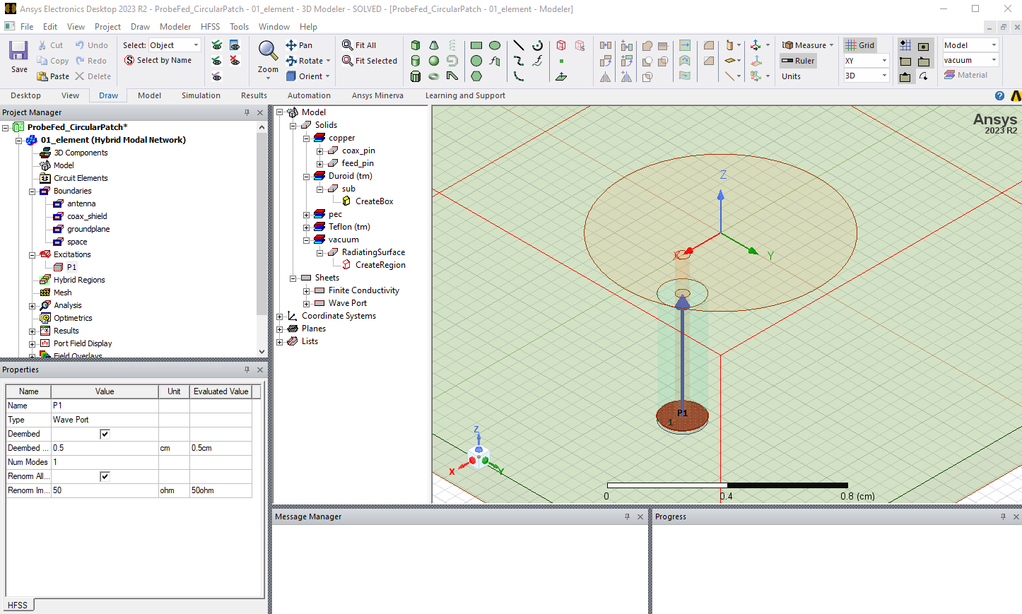
Wave ports are commonly used to simulate waveguide antennas and coax-fed antennas and to provide a 2D field solution, including the characteristic impedance and propagation constant. The port phase reference can be adjusted by de-embedding along the length of the feedline. Lumped ports can be used to provide a direct excitation at specific locations, such as between the arms of a dipole antenna. The user specifies the reference impedance for the impressed excitation.
The image below shows a wave port assigned to the coaxial cable that feeds the patch antenna. For this scenario, when a wave port is located within the model volume, a conducting object is used to back the port. The arrow denotes the de-embedding distance for the port definition.
Setting Up the HFSS Solution and Frequency Sweep
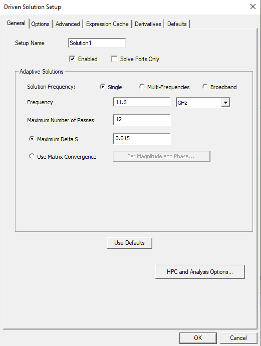
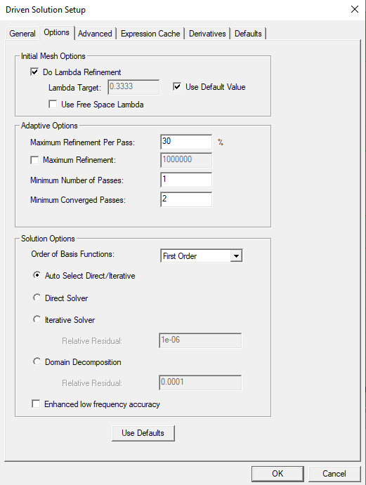
The final step before solving the model is specifying the solution parameters. This includes defining the adaptive meshing frequency, frequency sweep type, and resolution, as well as solution parameters related to convergence. The adaptive solution frequency can be specified at the highest frequency of interest to ensure a good mesh is obtained. The mesh can also be adapted to multiple specified frequencies or across a specified frequency band. The default convergence parameter for antenna models that include ports is the maximum difference in the S-parameter values between the current and previous adaptive pass. The image below on the left shows a solution set that adapts to mesh at 11.6 GHz until the change in S-parameter values falls below 1.5%. The Options tab is shown on the right with HFSS set to use the default first-order mesh elements and automatically select the most suitable matrix solver.
Adaptive Meshing and Convergence in HFSS
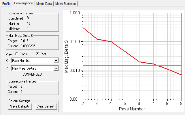
HFSS uses the finite element method to solve Maxwell’s equations and applies an adaptive meshing algorithm that intelligently adds mesh elements throughout the solution domain until the specified convergence criteria are reached. As shown in the image below, this patch antenna model completed 9 adaptive passes, with the final two passes meeting the 1.5% S-parameter convergence criterion. The solution time was 2 minutes on a standard desktop computer with 7 cores, and the final model contained approximately 41,000 tetrahedral mesh elements.
Understanding the HFSS Finite Element Mesh
HFSS employs an automatically adaptive meshing technique to efficiently and accurately simulate electromagnetic phenomena. This adaptive meshing capability specifies the local mesh density based on the electromagnetic field variations within the simulation domain. Additionally, HFSS provides users with control over mesh settings and refinement criteria as well as the ability to create mesh operations that enforce a certain mesh density in specified areas of the model.
An initial mesh is created based on the geometry and the lambda refinement value. As adaptive passes are completed, HFSS monitors the electromagnetic field distribution and refines the mesh in regions of high field variation. By concentrating computational resources in these critical areas, HFSS ensures that the simulation achieves the specified convergence requirement with the most efficient mesh.
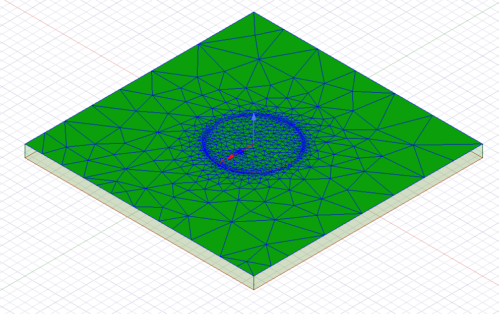
The image below shows the mesh that is automatically created by HFSS on the top surface of the patch antenna substrate. As expected, the edge of the circular patch is the most refined, since it is where the electromagnetic fields are concentrated in this type of antenna.
Analyzing S-Parameter Results for Impedance and Return Loss
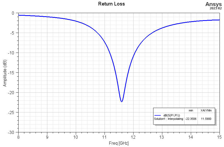
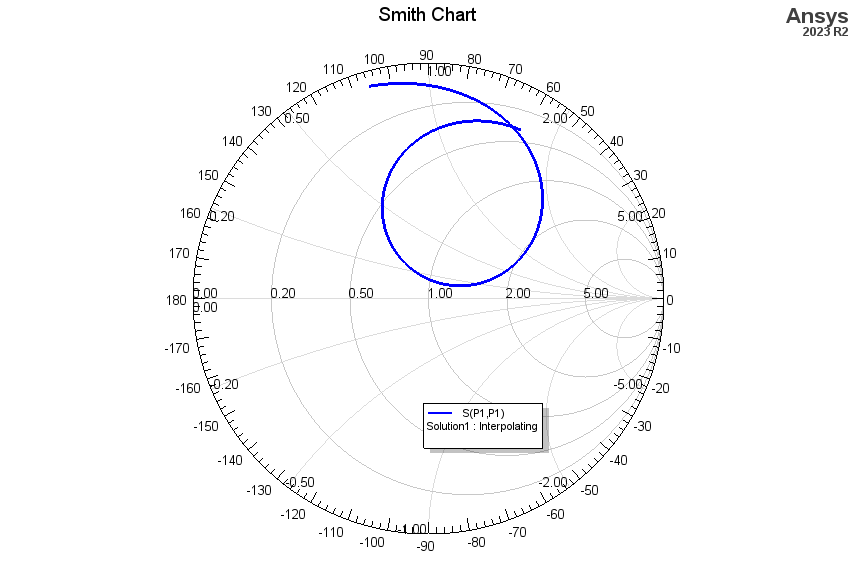
With HFSS, users can easily view S-parameters for the antenna structure. These parameters describe how electromagnetic signals propagate into the antenna and interact with connected components or transmission lines. By examining S-parameters, designers can assess performance metrics such as impedance matching, return loss, and bandwidth. Additionally, S-parameter analysis enables optimization of matching networks and feeding structures to enhance antenna efficiency and performance.
The plots below show the input return loss and impedance of the patch antenna model, showing a well-matched resonance at 11.59 GHz. The impedance response can be viewed on the Smith chart, where the center point corresponds to the impedance-matched condition.
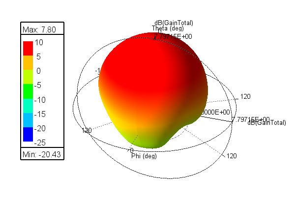
Viewing Far-Field Antenna Patterns and Gain
Viewing far-field results, such as antenna patterns and gain, helps antenna engineers understand the radiation characteristics and directional properties of their design. HFSS allows users to easily create a variety of 2D and 3D far-field plots and reports to assess important parameters, including directivity, gain, beamwidth, and radiation efficiency. This information can be used to optimize antenna designs to meet performance requirements. The images below show views of the far-field pattern, which can be overlaid onto the patch antenna geometry to indicate the direction of propagation.
Inspecting Near-Field Electromagnetic Distributions
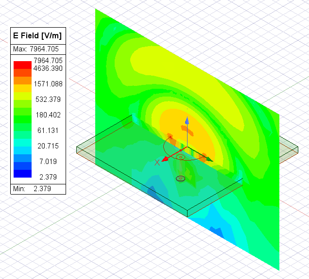
Users can also inspect the behavior of the electromagnetic field within the solution domain. This capability provides valuable insights into how electromagnetic waves interact with antenna structures and radiate into the surrounding environment. Users can visualize both the electric and magnetic fields in magnitude and vector formats, revealing how single- and multi-feed antennas generate radiating waves with the desired polarization.
HFSS enables users to animate the electromagnetic field solutions versus the phase for the time-harmonic solution, allowing for dynamic visualization of field propagation and interaction. This feature is useful to understand mutual coupling between antenna elements and other important phenomena in multi-antenna designs. By visualizing these electromagnetic field distributions and animations, users can identify design improvements and make informed decisions to achieve the desired performance goals.
The image below shows the magnitude of the electric field in the YZ plane for the circular patch antenna. The image is displayed on a logarithmic scale, and there are many options that allow the user to customize the plot’s appearance for presentations and reports. The field plot shows how the patch antenna radiates from the perimeter to produce a propagating wave centered on the patch.
This post outlined the HFSS antenna simulation workflow, from creating parameterized geometry to assigning materials and setting up boundary conditions. With appropriate port assignments, HFSS enables the extraction of S-parameters and input impedance. Adaptive meshing ensures efficient, accurate solutions, while far-field and near-field results provide insights into antenna performance. Watch the video below for a demonstration of the workflow.
Want expert guidance on your antenna design project? SimuTech Group offers Ansys HFSS training and consulting to help you get the most out of your electromagnetic simulations. Contact us to discuss your RF and antenna design challenges.