Zemax POP Fiber Coupling: Troubleshooting Incorrect Results

Introduction

In this example, we are given an existing Zemax OpticStudio file configured to evaluate fiber coupling using Physical Optics Propagation (POP). Rather than assuming the POP report is correct, we will begin by reviewing the results and asking a fundamental engineering question:

Is this result physically believable?

We will compare the POP behavior against what we expect from the optical system, look for inconsistencies in the beam propagation and reported data, and determine whether the model can be trusted. If something does not make sense, we will work through the problem systematically—using the geometrical model, pilot-beam information, sampling behavior, and POP settings to isolate the source of the error.

The goal is not simply to obtain a clean-looking POP plot. It is to develop a repeatable engineering workflow for determining when a POP result can actually be believed.

For an introduction to Physical Optics Propagation and the limitations of geometric ray tracing, see our earlier article, Zemax POP for Beginners: When Ray Tracing Is Not Enough for Laser Beams, before exploring this more advanced troubleshooting example.

Reviewing the Existing POP Result

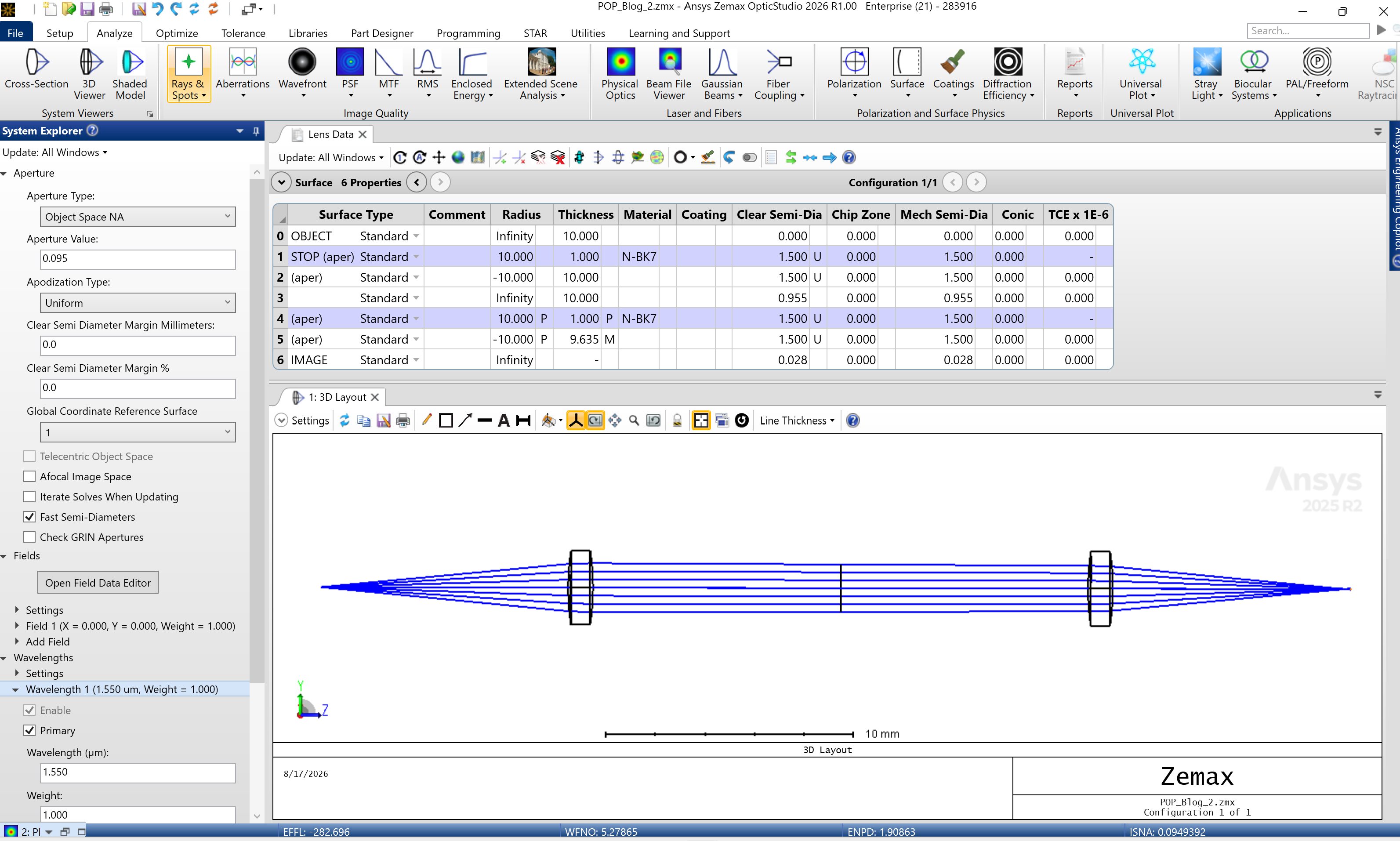
When we first open the file, the best place to start is keep the initial settings and study what the existing model is doing. The Lens Data Editor and 3D Layout show a simple fiber-coupling system: light begins at the object plane, propagates through the first lens, travels across the system, and is refocused by the second lens toward the image plane. The System Explorer defines an Object Space NA of 0.095 at a wavelength of 1.55 um. At first glance, the geometrical model behaves as expected – the rays expand from the source, are approximately collimated between the lenses, and converge again toward the image.

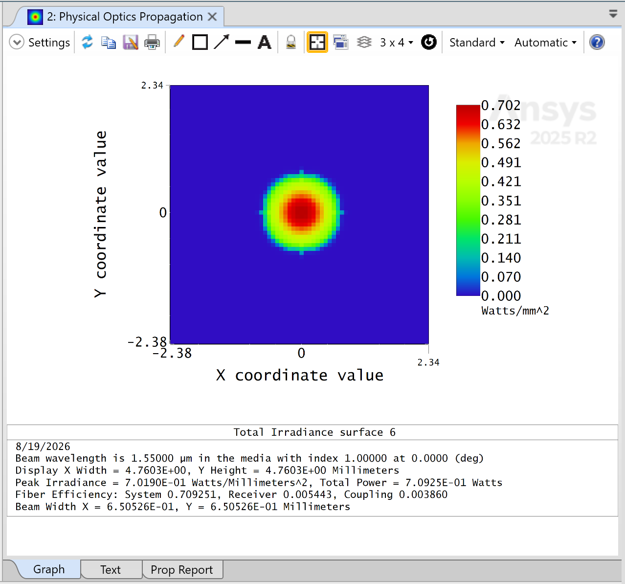
We can now compare that expectation with the existing POP result at Surface 6 above. Several immediate red flags suggest that we should NOT trust the POP results:

• Power is being lost. The POP calculation begins with 1 W of optical power, but only about 0.709 W reaches Surface 6, meaning nearly 30% of the power has disappeared somewhere in the propagation.
• The POP beam does not agree with the geometrical layout. The ray trace shows the beam converging toward a small image of 0.028 mm, while POP reports a beam width of approximately 0.651 mm at Surface 6. A full order of magnitude difference.
• The receiving fiber overlap is extremely poor. The reported receiver efficiency is only about 0.54%, producing an overall coupling efficiency of approximately 0.39% – which is bad.
• The beam spot in POP does not have a Gaussian Falloff. The beam looks clipped/vignetted somewhere because there is an abrupt falloff.

None of these observations tell us the cause yet. Aberration, clipping, sampling, or propagation settings could all affect POP calculations.

Finding Where the POP Result Goes Wrong

Rather than changing POP settings immediately, we can use the Beam File Viewer to inspect the propagated field at each surface. The goal is not yet to determine why the calculation is wrong, but to determine where the problem first appears.

In the Display Tab:

Check “Save Output Beam To:”

Check “Save Beam At All Surfaces”

We will review the Beam File Viewer surface by surface starting with Surface 1, the Starting Surface.

At each surface, we should ask:

• Does the beam size make sense compared with the geometrical rays?
• Does the beam still have the expected Gaussian profile?
• Is optical power being conserved?
• Does clipping or truncation suddenly appear?
• Does the reported pilot-beam behavior make physical sense?

The first surface where one of these quantities becomes inconsistent gives us a much smaller region of the model to investigate.

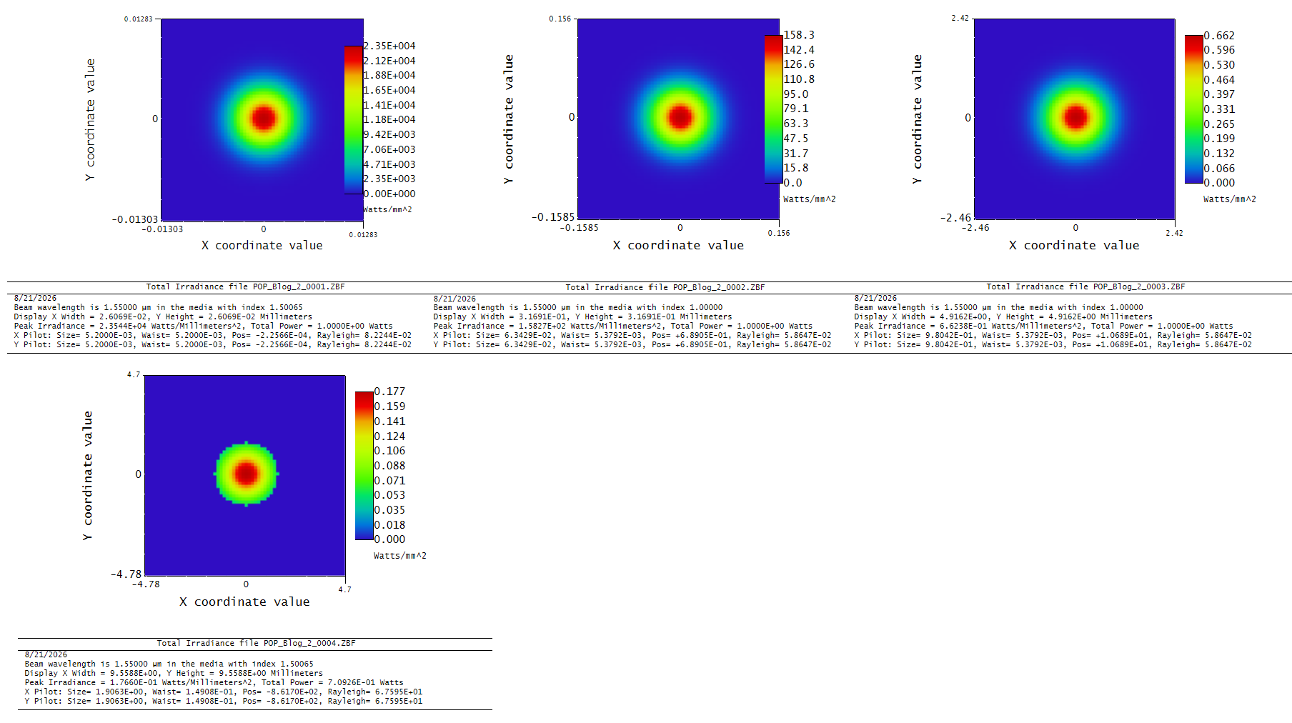
Starting with Surface 1, the beam propagation appears reasonable. The irradiance and lens distribution maintains a smooth Gaussian profile, the beam expands through the first lens, and the total power remains approximately constant. We have changed no settings, only zoom X8 to inspect the beam closer.

As we continue through the system, Surface 4 is the first location where a significant concern appears.

The most obvious issue is the abrupt edge in the irradiance distribution. A Gaussian beam should smoothly decay toward the edges, but the POP result shows a sharper cutoff behavior, suggesting that the beam may be interacting with an aperture or clear aperture limitation.

The power report provides additional evidence:

• The total power has decreased from the initial 1 W input.
• The beam appears larger than expected when compared with the physical size of the seco
• The abrupt falloff suggests that some of the beam energy may be clipped before reaching the final coupling surface.

At this point, the most reasonable engineering hypothesis is:

Is the second lens aperture too small for the propagated beam?

One possible solution would be to increase the physical size of the optics and rerun the analysis. However, before modifying the optical design, we should continue examining the remaining propagation surfaces.

A critical part of troubleshooting is avoiding premature changes. If the issue is caused by an incorrect model assumption or POP configuration, increasing the lens diameter may hide the real problem rather than solve it.

Therefore, we continue inspecting Surface 5 and Surface 6 to determine whether the beam behavior supports the aperture-clipping hypothesis.

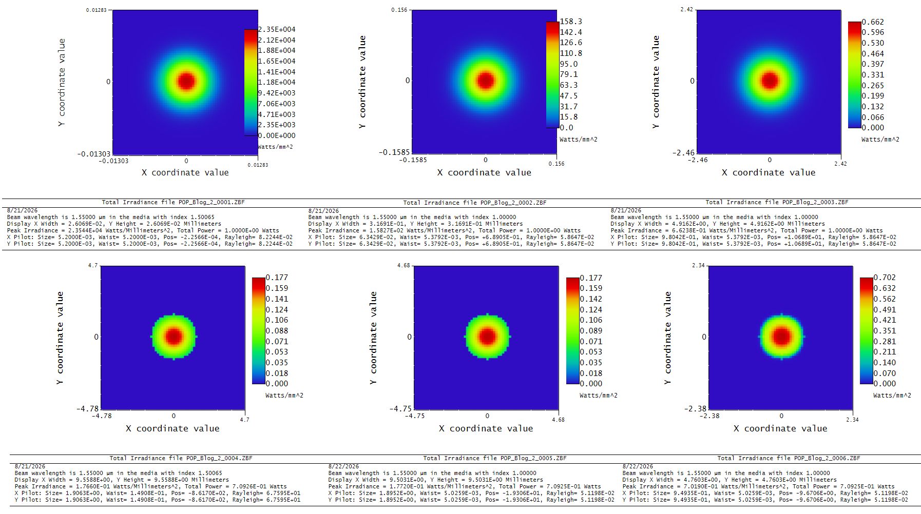
After identifying the abrupt truncation behavior at Surface 4, we continue examining the remaining propagation surfaces.

At Surface 5 and Surface 6, the important observation is that the clipping signature remains present. The beam is no longer a pure Gaussian beam; instead, we are observing the propagation of the clipped field created at Surface 4.

The propagation behavior provides several clues:

• The beam profile remains centered and symmetric, but the sharp truncation from Surface 4 continues to propagate.
• The irradiance distribution no longer represents the smooth Gaussian profile expected from an unclipped fundamental mode.
• The total power remains approximately constant after Surface 4, indicating that the majority of the power loss occurred at the clipping event rather than during propagation to the image plane.
• The beam continues to shrink as it propagates toward the focus, but the final field distribution is now determined by the diffraction of the clipped aperture.

This is an important distinction:

Once POP encounters clipping, the subsequent surfaces do not “recover” the original Gaussian beam. They propagate the modified electric field that remains after the aperture interaction.

At this point, our original hypothesis is still reasonable:

The beam appears to be larger than the available aperture, causing clipping at Surface 4.

The next question is therefore:

Why was the beam large enough to clip in the first place?

The next step is to look beyond the irradiance plots and examine the additional information provided by the Beam File Viewer. In particular, the reported pilot beam size, waist location, and Rayleigh range provide insight into how POP is interpreting the underlying Gaussian beam.

At Surface 5, the Beam File Viewer reports approximately:

• Pilot beam size: 1.895 mm
• Waist radius: 5.026 µm
• Waist position: −19.306 mm
• Rayleigh range: 0.05198 mm

At Surface 6, the Beam File Viewer reports approximately:

• Pilot beam size: 0.949 mm
• Waist radius: 5.026 µm
• Waist position: −9.671 mm
• Rayleigh range: 0.05198 mm

The beam size behavior itself is consistent: the beam is converging as it approaches the waist. However, the waist location immediately raises a concern.

The geometrical ray trace shows that the second lens should refocus the beam near the image/fiber plane. However, the POP pilot beam indicates that the Gaussian waist is still approximately 9.7 mm beyond Surface 6.

This is the first major inconsistency between the sequential model and the POP calculation.

The question changes from: “Is the second lens aperture too small?”

To: “Why does POP think the beam focus occurs at a different location than the geometrical model?”

The Root Cause: The POP Beam Definition Does Not Match the Geometrical Source

The next step is to review the POP initial beam definition.

This reveals an important concept when working with Physical Optics Propagation:

The Lens Data Editor and POP beam definition are related, but they are not the same thing.

The Lens Data Editor defines the sequential optical system:

• Object location
• Lens positions
• Radii
• Thicknesses
• Apertures
• Materials

However, POP requires its own definition of the input electric field:

• Beam type
• Beam size or waist
• Divergence
• Power
• Physical location of the beam relative to the POP start surface

A common misconception is that POP automatically knows the exact physical location of the Gaussian waist simply because the sequential model contains an object surface.

It does not.

In this example, the geometrical model defines the source at Surface 0, which is located 10 mm before the first lens.

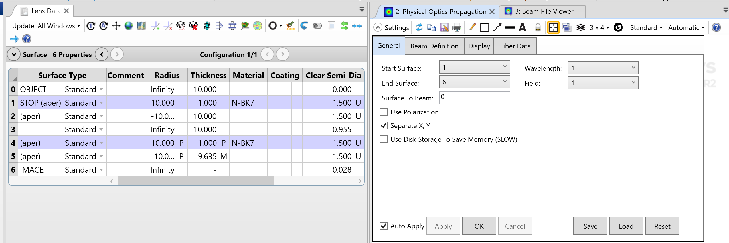
However, the POP calculation was started at Surface 1, and the initial Gaussian waist was placed at the starting surface.

This means POP was not propagating the same beam that was defined in the geometrical model.

The Gaussian waist size was correct — it matched the expected NA — but the axial location of the waist was incorrect.

The correction is therefore not to increase the lens diameter or adjust the POP sampling. The correction is to align the POP beam definition with the physical source location:

Surface To Beam = -10 mm

This places the POP waist at the same physical location as the geometrical object plane.

The hypothesis is that the POP beam was beginning at the first lens and therefore diverging all the way to Lens 2. That is why we clipped on Lens 2, Surface 4 of POP and that is why Position and Beam Parameters are not matching our Geometrical understanding. The fix is to realize the starting surface is Lens 1 and the beam needs to be set -10 mm in front of the Start Surface.

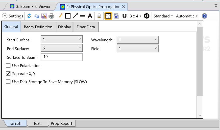
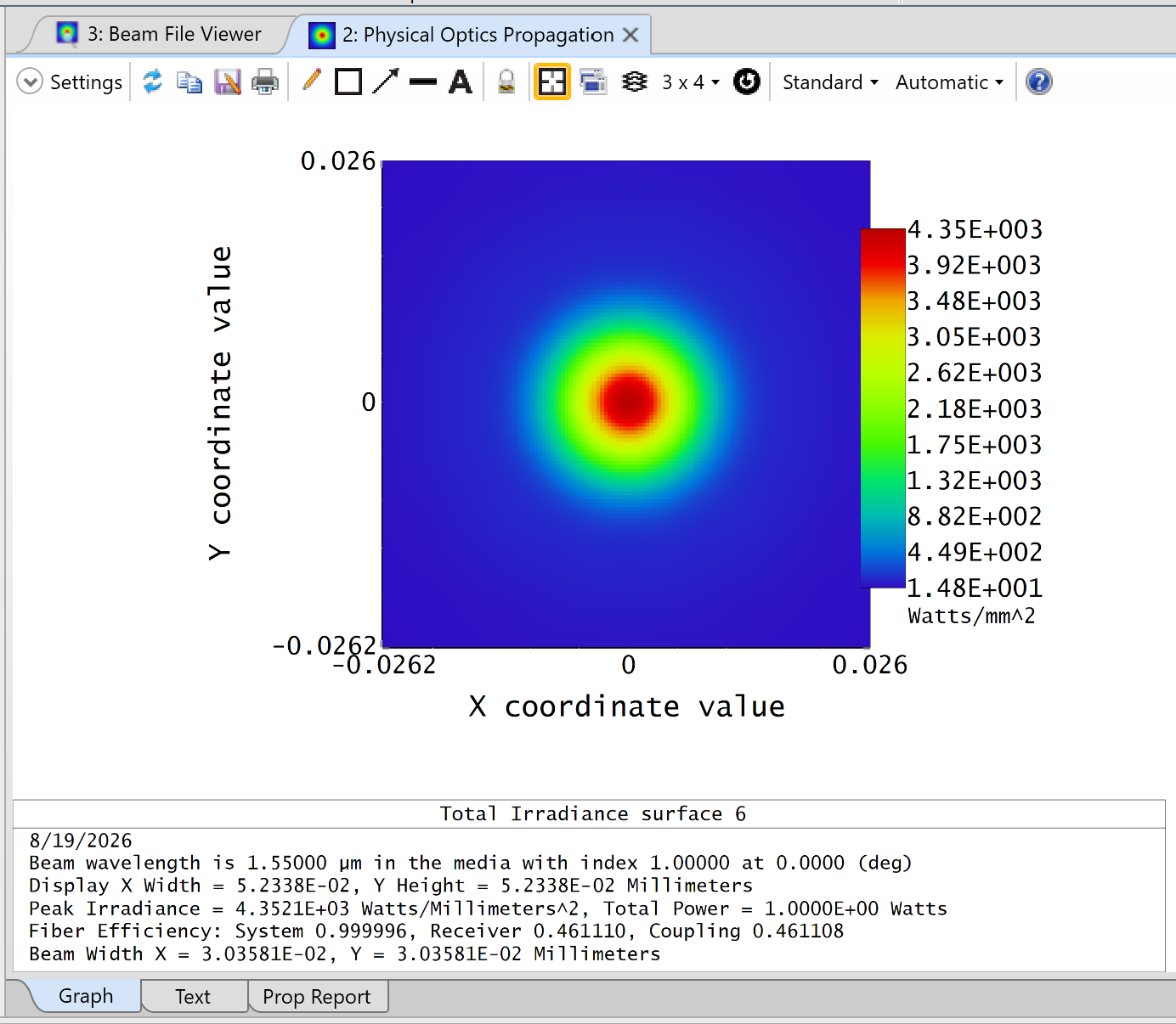
After correcting the initial condition, the clipping disappears, the beam focuses where expected, and the POP result becomes consistent with the sequential model.

The mistake was not in POP propagation. The mistake was assuming the Lens Data Editor and POP beam definition were automatically synchronized.

Explore Advanced Optical Simulation Training

Want to build your skills in optical propagation and fiber coupling? SimuTech Group offers specialized training, including OPTI 302: Ansys POP Analysis, covering beam definitions, diffraction, sampling, and troubleshooting, and OPTI 301: Co-Packaged Lumerical & Zemax, exploring integrated optical simulation and fiber coupling workflows.

Need Help Troubleshooting Your Optical Simulation Results?

Incorrect beam definitions, unexpected power loss, and poor fiber coupling predictions can make it difficult to trust your optical simulation results. SimuTech Group’s optical engineers can help you troubleshoot Ansys Zemax OpticStudio models, validate Physical Optics Propagation settings, and evaluate laser and fiber coupling performance.

Explore Our Optical Simulation Consulting Services to discuss your next project.