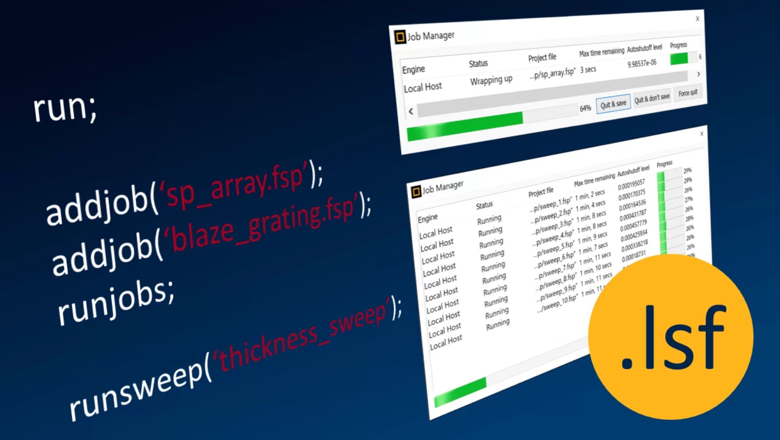
Ansys Lumerical Automation API for Python and L-Scripts
Ansys Lumerical Automation API Enablement
Enabling Lumerical tools to exchange data, in tandem with third-party applications, and a vast set of Python content.
• With Ansys Lumerical Automation API… Deploy Photonic Inverse Design capable of automatically identifying the best geometries for the necessary target performance.
• Run optical, thermal, and electrical simulations in a single file, then use Python to post-process the data.
• Create your own custom connectors and applications in-house.
• A large selection of Python libraries for mathematical analysis, visualization, optimization, and other uses.
• Explore powerful, open-source Python community projects.
Advancing Photonic & Circuit-Level Design with Lumerical Automation API.
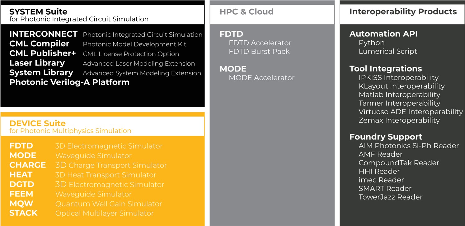
Ansys Lumerical Products
Designers can model interacting optical, electrical, and thermal effects thanks to tools that seamlessly integrate device and system level functionality. A variety of processes that combine device multiphysics and photonic circuit simulation with external design automation and productivity tools are made possible by flexible interoperability between products.
Ansys Lumerical MODE
Optical Waveguide & Coupler Solver
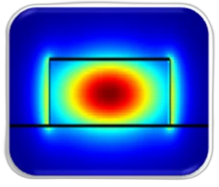
Engineers can reliably predict waveguide and coupler performance using MODE. Large planar structures and extended propagation lengths are no problem for MODE, which combines bidirectional Eigenmode expansion, varFDTD, and finite difference eigenmode solvers to deliver accurate spatial field, modal frequency, and overlap evaluations.
- Overlap Analysis
- Bend Loss Analysis
- Helical Waveguides
- 2.5D varFDTD Solver
- Anisotropic Materials
- Advanced Conformal Mesh
- Eigenmode Expansion Solver
- Spatially Varying Temperature
- Charge Density Profile Imports
- Finite Difference Eigenmode Solver
- Magneto-optical Waveguide Analysis
Advanced Bend Loss Analysis
Advanced bend loss analysis is offered by Lumerical MODE employing spectrally and spatially resolved imaging.
Rapid Overlap Calculation/Analysis’
To determine the differences and similarities between two or more databases or collections as well as the degree of overlap between resources, overlap calculation and analysis are simple to perform.
Modal Area Analysis
Multiple stages of analysis throughout the simulation process are necessary to get a reliable final design. With modal area analysis, Lumerical MODE accomplishes this feat.
Variational FDTD Solver
Enjoy the 3D FDTD accuracy while using 2D simulation times. The 2.5D varFDTD solver in Lumerical MODE can accurately and quickly model massive planar waveguides.
Bidirectional Eigenmode Expansion
To mimic electromagnetic propagation for long propagation lengths in waveguide or fiber devices, use the Lumerical MODE. Device length and periodicity are automatically surveyed by the software.
Ansys Lumerical FDTD
Simulation of Nanophotonic Devices
This expertly refined FDTD method (also known as Yee’s Method) offers best-in-class solver performance across a wide range of applications. The integrated design environment offers advanced post-processing, optimization, and scripting capabilities, allowing you to concentrate on your design while leaving the rest to Lumerical FDTD.
- Q-factor Analysis
- Band Structure Analysis
- Flexible Material Plug-ins
- Cloud and HPC Capability
- 2D or 3D Model Simulation
- Full Vectoral Customization
- Far-field Projection Analysis
- Spatially Varying Anisotropy
- Custom Surfaces and Volumes
- Advanced Conformal Meshing
- High NA Broadband Beam Sources
- Automated S-parameter Extraction
- Scripting and Optimization Routines
Photonic Inverse Design
- Automatically find the optimal geometries and designs for a specific design goal. Find counterintuitive geometries that enhance manufacturability, reduce area, and optimize performance.
Robust Post-Processing Analysis
- Far-field projection, band structure analysis, development of the bidirectional scattering distribution function (BSDF), Q-factor analysis, and charge production rate are only a few of the robust post-processing techniques available.
Anisotropy and Nonlinearity
- Simulate devices made from nonlinear or anisotropic materials that fluctuate spatially. Select from a variety of gain, negative index, and nonlinear models. Leverage adaptable material plug-ins, and define new material models.
Multi-coefficient Models
- Deploy multi-coefficient models to accurately simulate materials over a wide range of wavelengths. Source sample data (API configurability) to automatically develop models, or create your own procedures.
3D Computer-Aided Design Framework
- For both 2D and 3D models, FDTD’s CAD environment and parameterizable simulation components enable quick model iterations for engineers.
Lumerical INTERCONNECT
Photonic Integrated Circuit Simulator
The photonic integrated circuit simulator from Lumerical, INTERCONNECT, explores and evaluates multimode, bidirectional, and multi-channel PICs (Photonic Integrated Circuit). Engineer’s can use INTERCONNECT’s extensive library of primitive elements and foundry-specific PDK (Process Development Kit) elements when creating projects in the hierarchical schematic editor to conduct statistical analysis in the time or frequency domain.
- Transient Block Analysis
- Frequency Domain Analysis
- GUI and Lumerical Scripting
- Mixed Signal Representation
- Travelling Wave Laser Model
- Automatic Parameter Sweeps
- Multi-Variant Statistical Analysis
- Import Compact Libraries Models
- Electronic-Photonic Co-Simulation
- Transient Sample Model Simulator
- Multimode and Multichannel Support
Design and Simulation of PICs
- Use INTERCONNECT to create and simulate photonic integrated circuits using its hierarchical schematic editor.
- Frequency domain analysis, transient sample mode simulation, and transient block mode simulation are all included in INTERCONNECT.
- With support for parameter sweeps and design optimization, the software comes with comprehensive visualization and data analysis capabilities.
PDA and EDA Interoperability
- Use well-known EDA design tools and workflows to simulate and optimize your designs to shorten design cycles and increase reliability.
- PDA employs a two-level strategy that combines proactive, high-level system and product robustness assessments with rule-based “drill-down” probing to automatically gather comprehensive design-related data.
Variant Annotation & Statistical Analysis Solutions
- Use corner analysis to simulate how process variation affects the functionality of the circuit.
- Assess circuit performance and yield using Monte Carlo analysis while taking process variability into consideration.
PIC Element Libraries
- INTERCONNECT has a vast photonic integrated circuit (PIC) library. The library includes passive and active optoelectrical building components allowing users to customize their simulations.
CML Development and Dissemination
- INTERCONNECT offers an infrastructure that facilitates the creation and distribution of compact model libraries (CMLs) for PIC simulation and design, in addition to Ansys Lumerical’s device level tools.
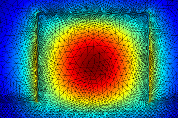
Ansys Lumerical CHARGE
3D Charge Transport Solver
The engineering tools for detailed charge transport simulation of active photonic and optoelectronic semiconductor devices are readily available in Lumerical CHARGE. The set of equations defining electrostatic potential (Poisson’s equations) and density of free carriers is self-consistently solved by CHARGE (drift-diffusion equations). State-of-the-Art simulation tools for automatic and guided mesh refining are leveraged by engineers to maximize accuracy while requiring the least amount of computational work.
- Scriptable Material Properties
- Automatic Finite Element Meshing
- Electrical/Thermal Material Models
- Parameterizable Simulation Objects
- Geometry-Linked Sources/Monitors
- Comprehensive SoC Material Models
- Small Signal Alternating Current analysis’
- Isothermal, Non-Isothermal, Electro-Thermal
Steady-state, Transient, Pole-Zero & Small-Signal AC simulation
Transient Analysis
A user-specified time interval is used to compute the transient output variables in Lumerical CHARGE transient analysis section. A DC analysis can automatically determine the beginning conditions. All sources (such as power supply) that are not time-dependent are set to their DC value. Initial conditions are assumed at the start of the analysis rather than the outcome of the DC operating point analysis if Josephson junctions are present or if the UIC option is specified. All sources should start with zero output in Josephson junctions. The transient simulation can be run at each point over a variety of bias settings by combining transient analysis with a DC sweep.
Transfer Function Analysis
The AC small signal transfer function, input impedance, and output impedance of a network are calculated by Lumerical HEAT’s transfer analysis section. The DC operating point for AC analysis is automatically calculated using an operating point analysis. Moreover, the transfer function can be estimated at each point over a variety of bias circumstances by combining the transfer analysis with a DC sweep.
Pole-Zero Analysis
The poles and/or zeros in the small-signal AC transfer function are computed by the pole-zero analysis section of Lumerical CHARGE. All of the nonlinear components in the circuit’s linearized, small-signal models are then determined after the DC operating point has been calculated. The poles and zeros are then determined using this circuit. The transfer functions (output voltage)/(input voltage) and/or (output voltage)/(input current) are readily accessible for engineers to employ.
The poles and zeros of functions like input/output impedance and voltage gain can be found using these two forms of transfer functions, which cover all circumstances. With resistors, capacitors, inductors, linear-controlled sources, independent sources, BJTs, MOSFETs, JFETs, and diodes, the pole-zero analysis can be applied.
Small Signal AC Simulation
The AC output variables are calculated as a function of frequency by the AC small-signal section of Lumerical HEAT. The program initially calculates the circuit’s DC operating point before determining linearized, small-signal models for each of the circuit’s nonlinear components. The resulting linear circuit is next examined across a user-specified frequency range. Typically, a transfer function is the desired result of an AC small-signal analysis (voltage gain, transimpedance, etc). If there is just one AC input in the circuit, it is practical to set it to unity and zero phase such that the output variables have the same value as their transfer function to the input. A DC sweep and AC analysis can then be used in tandem to perform an alternating current analysis at each position under various bias conditions.
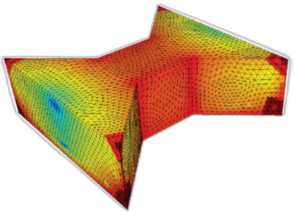
Ansys Lumerical HEAT
3D Heat Transport Solver
Deploy Lumerical HEAT to reliably, and systematically, address your engineer’s needs for heat simulation. A finite-element heat transfer and Joule heating solver are included in the 3D heat transfer simulation to emulate the thermal conductive, convective, and radiative effects on the optical properties of your device.
- Joule (J) Heating Solver
- Flexible Materials Database
- Automatic Mesh Refinement
- Finite-Element Meshing Automation
- Finite-Element Heat Transport Solver
- Steady-State and Transient Simulation
- Rapid Transition from 2D & 3D Solvers
- Self-Consistent Heat/Charge Transport
- Conductive, Convection & Radiative Effects
Heat Transport Solver Simulations
For steady-state and transient simulation, Lumerical HEAT provides a 2D/3D finite element heat transfer solver.
- Automatic mesh refinement
- Joule heating via electrical conduction
- Comprehensive models for thermal materials
- Heat flux, convection and radiation analysis
- Automatic Programming Interface transfer for heat profiles
Highly Integrated Interoperable Solvers
Self-consistent charge and heat transport simulation is offered by Lumerical HEAT. HEAT can be used in tandem with other Lumerical solutions to conduct multiphysics simulations:
- Photovoltaic (FDTD/DGTD, CHARGE & HEAT)
- Opto-thermal (FDTD/DGTD & HEAT)
- Plasmonics (DGTD & HEAT)
Self-Consistent Charge/Heat Modeling
Flexible implementation capable of capturing thermal optical and electro-optical effects.
- Self-heating effects and property-based variations
- High-current electronic, photonics and optical devices
FE Interactive Design Engineering
Automatic mesh refinement catered to Finite Element IDE, based on geometry, materials, doping, refractive index, and optical or heat generation.
- Dual 2D & 3D modeling
- Import STL, GDSII, and STEP
- Parameterizable simulation components
- Geometry-linked sources and monitors for presets
- Domain partitioned solids for seamless property definition
Comprehensive Material Models
With more than 500 adjustable electronic and thermal properties, the material database enables precise modeling of complicated effects, and scriptable material properties, Lumerical HEAT offers a flexible visual database.
Ansys Lumerical DGTD
3D Electromagnetic (EM) Simulator
The core engineering framework of 3D electromagnetic simulations in Lumerical DGTD are accuracy and performance. A finite element Maxwell’s solution based on the discontinuous Galerkin time domain approach is deployed to handle the most difficult classes of nanophotonic simulations. The powerful solvers offered by DGTD (Discontinuous Galerkin Time Domain) can be used to model and optimize new designs in a variety of fields, such as magneto-optics, augmented reality, micro-LEDs, and lasers.
- Highly Interoperable
- Object-Conformal Mesh
- Material-Adaptive Mesh
- Gaussian Vector Beams
- Automation and Scripting
- Bloch Boundary Conditions
- Automatic Mesh Refinement
- High Order Mesh Polynomials
- Transitional 2D & 3D Modeling
- Far-field and Grating Projections
Gaussian Beam Propagation
- In many laser optics applications, the laser beam is taken to be Gaussian with an optimal Gaussian distribution for the irradiance profile.
- For this reason, Lumerical DGTD has incorporated equations and other parameters that engineers will need to calculate the laser’s divergence from perfect Gaussian behavior.
- The M2 factor, also known as the beam quality factor, contrasts a real laser beam’s performance with a diffraction-limited Gaussian beam.
- Custom Gaussian irradiance profiles can be created using DGTD, enabling symmetry analyses around COB distances to measure directional propagation increases.
Bloch Boundary Conditions (BC’s)
- Lumerical DGTD enables seamless phase correction when simulating a plane wave propagating at a specified angle.
- Bloch boundary conditions are employed in a number of settings, but they are most frequently used in simulations of periodic structures illuminated by an angled plane wave source.
- When determining the in-plane wavevector is important, Bloch Boundary Conditions (BCs) are crucial in contextualizing results. For instance, they are routinely utilized by photonics engineers in Bandstructure computations.
Interoperable with Multiphysics Solvers
Several multiphysics simulations are offered by Ansys Lumerical DGTD in addition to other Lumerical solutions:
- Photovoltaic (FDTD/DGTD, CHARGE & HEAT)
- Electro-optic (CHARGE & FDTD/DGTD/FDE)
- Opto-thermal (FDTD/DGTD & HEAT)
- Plasmonics (DGTD & HEAT)]
Optical Phase Change Materials with Broadband Transparency
- Designers frequently assume that isoelectronic substitution will tend to widen the optical bandgap, which will reduce the near-infrared interband absorption.
- One of the main embedded solutions with Lumerical DGTD is the impact of replacement, which determines the optical loss in the mid-infrared.
- Engineers can discover impressive low-loss performance advantages from blue-shifted interband transitions and minimum FCA through proper deployment, which is supported by linked first-principle modeling and experimental characterization.
- Utilizing the exceptional optical features of this innovative solution provided by DGTD, record low losses in non-volatile photonic circuits and electrical pixelated switching can be identified.
- In addition, Lumerical DGTD offers a flexible visual database, with multi-coefficient broadband optical material models and scriptable material properties.
Ansys Lumerical FEEM
Finite Element Waveguide Simulation
Lumerical FEEM’s finite element Maxwell’s solver, which is based on the Eigenmode expansion algorithm, offers superior accuracy and performance scaling. Seamlessly calculate and analyze the modes that the 2D cross-section of waveguides or fibers can support in the frequency range.
- Frequency Domain Reflectometry
- Higher-Order Polynomial Functions
- Parallel Curved Meshing Simulation
- Spatially Varying Index Perturbations
- Determine Effective Refractive Index’
- Fourier analysis for Signal Processing
- Material-adaptive Mesh Embedment
- Electro-Optic/Thermo-Optic Modeling
- Waveguide Thermal Sensitivity Tuning
Frequency Domain Reflectometry (FDR)
Optically propagate a signal through a metal tine or another wave path in Ansys FEEM by seamlessly deploying oscillators. To gauge soil moisture, the difference in frequency between the output wave and the return wave is monitored.
Traditional time domain reflectometry (TDR), which is best suited for locating open and short circuit situations in conductors, may not be as sensitive to cable degradation as the FDR method due to its inherent benefits.
Because there are filtering and noise-reducing techniques in the frequency domain, for instance, FDR is less vulnerable to electrical noise and interference. Increased sensitivity and accuracy may result from this.
Additionally, since TDR pulses may have trouble moving forward after numerous noteworthy reflections, FDR analysis in FEEM is better suited for locating and describing a series of multiple deterioration episodes in lengthy cables.
Fourier Analysis for Signal Processing
In Ansys FEEM, The Fourier Transform and Plot/Modify Input Signal dialog boxes allow engineers to set several different functions for the x and y axes, apply different FFT windowing techniques, and set various output options.
Acting as a tool for signal decomposition for further filtration, engineers can visualize the material separation of the various signal components. This process of bridging the gap between these two worlds (time and frequency domain) is paramount to RF engineers.
Engineers can easily apply the various Discrete Fourier Transform calculation methods using FEEM, starting with the application of the Fourier Transform, moving on to the simplified calculation technique, and concluding with the Cooley-Tukey method of the Fast Fourier Transform.
Spatially Varying Index Perturbations
Engineers can use the (n,k) Material import object in Ansys FEEM to transform spatially variable stress or strain into a spatially variable refractive index profile.
It is crucial to distinguish between circumstances that will cause diagonal anisotropy and those that won’t when introducing the spatially variable refractive index owing to stress or strain. Using a nk import material, which is accessible in Ansys FEEM, FDTD, and MODE, it is simple to address the diagonal anisotropy that is the focus of this example.
It will be essential to diagonalize the permittivity tensor and perform a matrix transformation to add the influence of the strain if the stress or strain produces a permittivity tensor with off-diagonal elements. Matrix transformation makes it simple to set up the matrix transform grid properties and specific stress inputs while also providing engineers with visual assistance to help them choose the best application.
Ansys Lumerical MQW
Quantum Well Gain Simulation
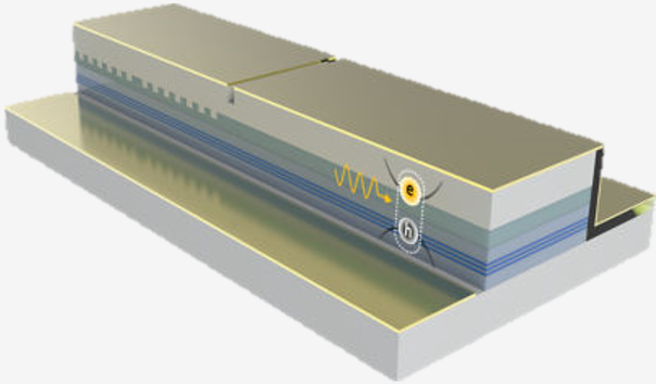
Band structure, gain, and spontaneous emission across multi-quantum well architectures can be quantitatively characterized by simulating quantum mechanical activity in atomically thin semiconductor layers. To enable the construction of lasers, SOAs, electro-absorption modulators, and other gain-driven active devices, MQW couples to Lumerical CHARGE, MODE, and INTERCONNECT.
- Wavefunction Calculation
- Band Diagram Calculation
- Physics-Based Photonics Solver
- Quantum Mechanical Analysis
- Conduction Electron Scattering
- Gain and Spontaneous Emission
- Comprehensive Material Models
- Characterization of Band Structures
- Temperature, Field and Strain Effects
- Multi-Quantum Well Stacks Simulator
- Establish Controllable Quantum States
- Mesoscopic Superconductivity Analysis
MQW Gain
Engineers can effectively measure band structure, gain, and spontaneous emission in multi-quantum well devices thanks to Ansys Lumerical MQW, which simulates quantum mechanical activity in atomically thin semiconductor layers.
Additionally, MQW offers a fully-coupled k.p approach calculation of the quantum mechanical band structure.
Dynamic Laser Simulation & Modeling
Produce dynamic laser models that incorporate tuning and outside feedback effects into account, simulate and extract important TWLM (Travelling Wave Laser Model) parameters, and analyze steady-state and transient laser performance.
The design and manufacture of MQW lasers are typically complex and expensive; hence, simulations can speed up development and provide information on design factors.
Additionally, when the parameters are changed, measured curves and simulated power curves can be contrasted. It is possible to closely analyze issues like nonradiative recombination and self-heating that affect how well the simulated laser works.
Mesoscopic Superconductivity
Engineers utilizing MQW can use the time-dependent Ginzburg-Landau equations to numerically solve the mesoscopic superconducting ring constructions (through finite-element analysis).
Mimic the dynamic behavior of complex magnetic vortices in the semiconductor for a given applied magnetic field.
Users can also look into the many vortex configurations, pinpoint the best vortex states using the two stable vortex shells in the mesoscopic superconducting ring. And finally, assess the improved photonic surface superconductivity.
Ansys Lumerical STACK
Optical Thin-Film Simulation
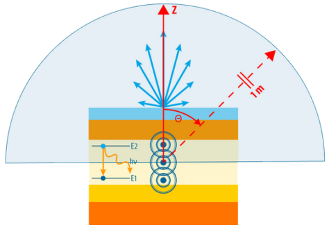
With Lumerical STACK, thin film stacks can be designed quickly. STACK is faster than direct simulations of the Maxwell’s equations since it makes use of analytical techniques. Interference and microactivity effects are accurately captured by the various thin film, photonic modeling software features under both plane-wave and dipole illumination.
- Plane-Wave Illumination
- Capture Interference Effects
- Capture Microactivity Effects
- Optical Thin-Film Application
- Dipole/Dipole Off-Axis Illumination
- Simulate Thin Film Multilayer Stacks
STACK Analytic Solver
In comparison to a direct simulation of Maxwell’s equations, the STACK Analytic solver is quicker. It has functionality for both plane-wave and dipole illumination and is excellent for rapid prototyping for thin film applications. Interference and microcavity effects are captured by the solver.
Scripting-based interoperability
Through the Automation API, Python and MATLAB APIs, as well as the Lumerical scripting language, Lumerical STACK products are flexible and easy to integrate into workflows.
Dipole/Dipole Off-Axis Illumination
Seamless transition between on-axis and off-axis illumination is available for engineers in Ansys STACK who often toggle between multiple resolutions and proximity corrections.
One of the three main resolution-enhancement technologies, off-axis illumination (OAI), has allowed optical lithography to push the practical resolution limitations well beyond what was previously thought to be conceivable (the others being phase shifting masks and optical proximity corrections). Off-axis lighting must be properly sized and shaped for the particular mask pattern being printed in order to be used efficiently for engineers in this line of work.