APDL Commands Objects in Mechanical Workbench After Response Spectrum Analysis

Using APDL Commands Objects in Postprocessing to Extract Data and Create Output Parameters

Ansys Mechanical Workbench supports Response Spectrum Analysis. Either single-point or multi-point response spectrum analysis can be performed. Depending on the results requested in Analysis Settings for a Response Spectrum solution, velocity and acceleration results can be obtained, in addition to deflection, stress and strain.

Users sometimes want to use APDL Commands Objects in postprocessing to extract results data and create Output Parameters. This article illustrates where information can be obtained with postprocessing APDL Commands Objects after a Response Spectrum Analysis.

Response Spectrum Analysis | Model Settings

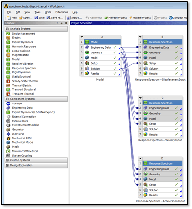
In a Response Spectrum Analysis, Workbench Mechanical permits description of supports (zero displacement boundary conditions) in the Modal environment. In single-point response spectrum analysis, an excitation input of Response Spectrum Displacement, or Velocity, or Acceleration can be added as an object in a Response Spectrum environment.

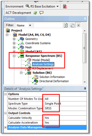
A global direction for the excitation is entered, and it is applied to all constrained nodes during the SOLVE. Analysis Settings can be used to indicate whether in addition to the displacement that is automatically generated, a user would like to have Velocity and/or Acceleration results generated:

Simulation APDL Commands Objects in Mechanical Workbench After Response Spectrum Analysis SimuTech Group

SimuTech Group APDL Commands Objects in Mechanical Workbench After Response Spectrum Analysis

Response Spectrum Analysis | Ansys Batch Run

During the Batch Ansys run that reads in the ds.dat file generated for an environment by Workbench Mechanical, results are saved in the RST results file in the folder for the environment. Examination of v14.5 models shows that with a Response Spectrum Analysis, the displacement results are saved in the RST file as Load Step 4, Substep 1. Velocity results are saved in Load Step 4, Substep 2. Acceleration results are saved in Load Step 4, Substep 3.

The structure of an example ds.dat file for a Response Spectrum analysis illustrates the formation of the Displacement, Velocity and Acceleration results. In the following example, Displacement, Velocity and Acceleration results have all been requested in Analysis Settings. Four code fragments of the ds.dat file are shown.

The reswrite command in the ds.dat file appends the result in database memory to whichever RST file is specified.

In the first code fragment taken from the ds.dat file, we see a SOLVE for a displacement analysis. After the MCOM file’s commands are executed (they combine the mode shapes into a combined response), the result is written to a new file called Temp.rst as Load Step 4, Substep 1:

/solu
antype,spectr
spopt,sprs
/copy,file,mode,,original,mode
SED,0,1,0
SVTYPE,3
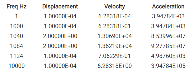
FREQ,1.,1000.,1040.,1084.,1124.,10000.
SV,,1.e-004,1.e-004,2.,2.,1.e-004,1.e-004
srss,0.0,disp
solve
freq
fini
*list,,mcom
/copy,file,mcom,,Displacement,mcom
/post1
/inp,,mcom
reswrite,Temp,4,1
fini
/copy,original,mode,,file,mode

In the second code fragment from the ds.dat file, Velocities result. After the MCOM file is executed, the result is appended to Temp.rst as Load Step 4, Substep 2:

/solu
SED,0,1,0
SVTYPE,3
FREQ,1.,1000.,1040.,1084.,1124.,10000.
SV,,1.e-004,1.e-004,2.,2.,1.e-004,1.e-004
srss,0.0,velo
solve
freq
fini
*list,,mcom
/copy,file,mcom,,Velocity,mcom
/post1
/inp,,mcom
reswrite,Temp,4,2
fini
/copy,original,mode,,file,mode

In the third code fragment from the ds.dat file, Accelerations result. After the MCOM file is executed, the result is appended to Temp.rst as Load Step 4, Substep 3.

/solu
SED,0,1,0
SVTYPE,3
FREQ,1.,1000.,1040.,1084.,1124.,10000.
SV,,1.e-004,1.e-004,2.,2.,1.e-004,1.e-004
srss,0.0,acel
solve
freq
fini
*list,,mcom
/copy,file,mcom,,Acceleration,mcom
/post1
/inp,,mcom
reswrite,Temp,4,3
fini
/DELETE,original,mode

In the last code fragment from ds.dat, the “usual” results file called file.rst is created by renaming Temp.rst:

/DELETE,file,rst
/RENAME,Temp,rst,,file,rst

Adding Velocity and Acceleration Results in Ansys Postprocessing

The RST results file available for postprocessing contains only one load step, numbered 4, with up to 3 substeps containing Displacement, plus Velocity and Acceleration results if requested in Analysis Settings. The historical reason for using Load Step 4 is not apparent, but may be related to older techniques employed in the ANSYS Mechanical APDL interface.

The Displacement result in Load Step 4, Substep 1 contains degree of freedom displacement results at nodes, in addition to derived stress and strain data. The Velocity result in Load Step 4, Substep 2 contains velocities instead of displacements as the “displacement” results at nodes, while the derived results (stress, strain etc.) are not physically meaningful. The Acceleration result in Load Step 4, Substep 3 contains accelerations instead of displacement at nodes, and again the derived results are not physically meaningful.

Response Spectrum Analysis | Deformation Plotting

The following figure shows a deformation plot resulting from a Response Spectrum analysis:

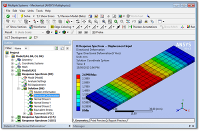
Understanding the above image requires examining Details settings for various objects in the Outline.

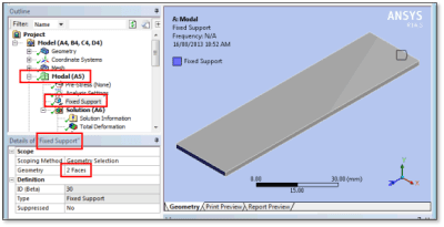
The Modal analysis included fixed supports at two ends of the plate in this model. More than enough modes of vibration were extracted to span the range of excitation frequencies used later.

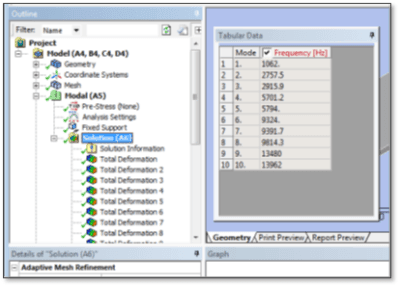
The natural frequencies of vibration calculated in the Modal environment are listed in a table:

Analysis Settings in the example Response Spectrum analysis requested a relatively simplified SRSS mode combination, and ignored more sophisticated settings that might be considered in accurate commercial work, for example:

Modes with closely-spaced natural frequencies.
Modes with partially- or fully-rigid responses.
High-frequency mode effects without extracting all modes.

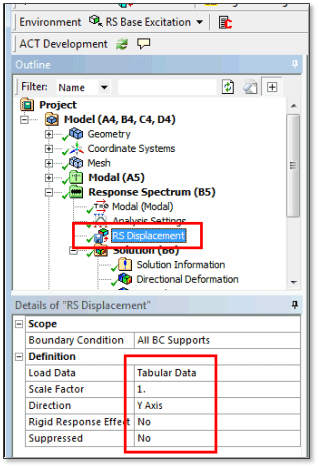
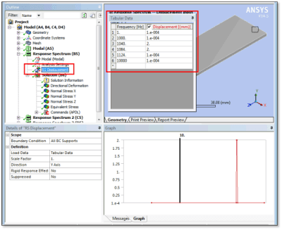
A Response Spectrum input of Displacement is entered to excite the structure in this example.

Modal Vibration Analysis & Determination of Peak Excitation

Data is entered in a frequency/amplitude table, taking care to employ the correct units and scale factor. Note that the region of peak excitation in this table spans the first mode of vibration in the Modal analysis above.

Results should include displacement plots, particularly in the direction of excitation, but should generally be created in X, Y and Z, as well as scoped to geometries of interest. Stress and strain results may be of interest.

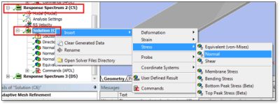
If Velocity and Acceleration were requested in Analysis Settings, they can be plotted, too:

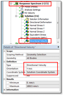
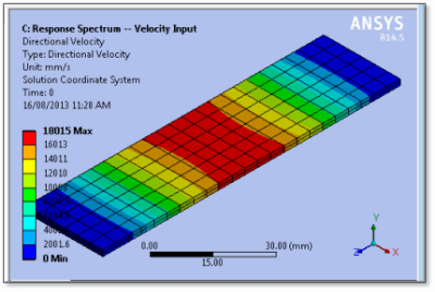
Velocity and Acceleration inputs are supported, as alternatives to a Displacement excitation in a single-point Response Spectrum analysis. A small spreadsheet was created to illustrate equivalent excitations when using Displacement, Velocity and Acceleration inputs. Velocity is Displacement multiplied by ω, and Acceleration is Velocity multiplied by ω. Displacements are in mm:

The same results were found for the test model whichever one of these three forms of excitation was applied. The figure above shows various results of interest after the Solution object for the Response Spectrum analysis. In addition to plotting these quantities, APDL commands can be used to get more information.

Results with APDL Commands Objects

The figure above shows an APDL Commands Object that contains the following APDL commands. They perform the following steps, with results printed in the solve.out file generated for the run. Possible contents are:

/COM, #####################################################################
/COM, #####################################################################
/COM, APDL Commands for Post Processing after Response Spectrum ###########
/COM, #####################################################################
/COM, #####################################################################
/COM, .
set,list ! Examine the RST file results in the output file
/show,png ! Generate plots in PNG format… display in Outline
/view,1,1,1,1 ! Isometric view
/gfile,600 ! Image height in pixels (borders are added to this)
!
plnsol,s,z ! Plot of Sz
plnsol,s,eqv ! Plot of Seqv
!
nsort,s,z ! Sort on Sz values
*get,my_stress_z_max,sort,,max ! Max Sz value from selected nodes sort
*get,my_stress_z_min,sort,,min ! Min Sz value from selected nodes sort
*get,my_stress_z_imax,sort,,imax ! Node with Max Sz
*get,my_stress_z_imin,sort,,imin ! Node with Min Sz

The above APDL coding example (not recommended) does NOT contain a SET command that reads in a result of interest. If there is no expansion of Velocity or Acceleration results, then when these commands execute they use the result in the Ansys in-memory database, which will be a displacement result.

Last Generated In-Memory Database Hierarchy

However, if a Velocity and/or Acceleration result has been expanded, then whichever was generated last will be in database memory, and the derived stress results extracted above will not be physically meaningful.

The set,list command included above will result in the following list of RST file information in the solve.out file when all of Displacement, Velocity and Acceleration have been requested:

***** INDEX OF DATA SETS ON RESULTS FILE *****

SET TIME/FREQ LOAD STEP SUBSTEP CUMULATIVE
1 0.0000 4 1 0
2 0.0000 4 2 0
3 0.0000 4 3 0

All results are considered to be Load Step 4. The Displacement, Velocity and Acceleration results are in Substep numbers 1, 2, and 3 respectively. To extract Displacement results and associated stress and strain results, a SET command must be employed:

set,4,1 ! Load displacement result and associated stresses and strains

After the SET command is used (preferred approach), the results of interest can be explored, for example:

/COM, APDL Commands for Post Processing after Response Spectrum ###########
/COM, .
set,list ! Examine the RST file results in the output file
/show,png ! Generate plots in PNG format… display in Outline
/view,1,1,1,1 ! Isometric view
/gfile,600 ! Image height in pixels (borders are added to this)
!
set,4,1 ! Access deflection and derived stress/strain results <———-
plnsol,u,y ! Contour plot of UY values
plnsol,s,x ! Contour plot of Sx
plnsol,s,y ! Contour plot of Sy
plnsol,s,z ! Contour plot of Sz
plnsol,s,eqv ! Contour plot of Seqv
nsort,s,z ! Sort on Sz results
*get,my_stress_z_max,sort,,max ! Max stress value from preceding sort
*get,my_stress_z_min,sort,,min ! Min stress value from preceding sort

After the nsort command, note the *get commands that retrieve max and min results of interest. *get can retrieve data on degree of freedom values, stresses, strains, and anything else generated in the RST file.

If set,4,2 or set,4,3 are issued, then the “apparent” displacement degree of freedom values will contain velocity or acceleration data, respectively. (The Analysis Settings must be set to non-default generation of Velocity and Acceleration for the data to be available).

Command DOF Result Meaning
SET,4,1 Displacement
SET,4,2 Velocity
SET,4,3 Acceleration

Note that postprocessing with APDL Commands Objects in Workbench can create Output parameters for Workbench if the parameter names start with the letters “my_”. Remember that when a Velocity or Acceleration result is loaded in APDL, derived data such as stress and strain have no physical meaning.

Conclusions | Mechanical Single-point and Multi-point Response Spectrum Analysis

Workbench Mechanical can perform both single-point and multi-point Response Spectrum analysis. The RST results file from such an analysis will contain the Displacement result in Load Step 4, Substep 1. If Velocity or Acceleration have been generated (non-default selections in Analysis Settings), they are saved in Load Step 4, Substep 2 and Load Step 4, Substep 3, respectively.

Once a SET command has loaded the result of interest from the RST file, plots can be generated with APDL commands, and use of the *GET or *VGET commands can move data of interest into parameters. This can permit customized postprocessing and design studies.

This simplified example used SRSS for mode combination. Professional analysis work may require more advanced Response Spectrum Analysis Settings. The purpose of this article was to illustrate results retrieval with APDL.