How to Create Reduced Order Models for Electronics Cooling with Ansys Icepak and Twin Builder

Introduction to Reduced Order Models

Reduced Order Models (ROMs) are a powerful way to bring high-fidelity thermal simulation results into fast system-level studies. In this blog, we will explain how to create ROMs for electronics cooling applications using Ansys Icepak and Ansys Twin Builder. The workflow starts with setting up the thermal Computational Fluid Dynamics (CFD) model in Icepak, extracting the required response data, and then using that information in Twin Builder to build compact models that can be used for transient thermal analysis, system simulation, and design exploration. We will also discuss the difference between the Linear Time-Invariant (LTI) ROM and the Linear Parameter-Varying (LPV) ROM available in Ansys Icepak, including when each approach is more appropriate.

Reduced Order Models in Electronics Cooling

In electronics cooling, engineers often need to evaluate thermal behavior across many operating conditions, power profiles, and design configurations. Full 3D CFD simulations are very accurate, but they can be computationally expensive, especially when transient simulations or system-level interactions are required. ROMs help solve this challenge by capturing the dominant thermal behavior and converting it into a much faster representation. This allows engineers to predict temperatures, thermal time constants, and heat-transfer interactions in seconds or minutes instead of running a full CFD simulation every time.

ROMs are especially important when the thermal model needs to be connected with electrical, control, or system-level models. For example, a ROM of a power electronics module can be used in Twin Builder to predict junction temperatures under different input conditions, such as variable load cycles in an inverter or motor drive. Another common example is a server or electronic enclosure, where ROMs can be used to evaluate how component temperatures respond to changes in inlet flow and power dissipation. In both cases, the ROM preserves the key thermal behavior of the detailed CFD model while enabling fast simulation of many scenarios.

Instead of solving the full Icepak model repeatedly, an LTI or LPV ROM can be used to rapidly estimate component temperatures for different power inputs. This makes ROMs valuable not only for design validation, but also for optimization, digital twins, and real-time thermal monitoring.

Icepak ROM General Workflow

The purpose of this blog is to show the steps required to generate a ROM using Icepak and Twin Builder. The ROM created in this workflow is a transient system-level reduced order model. This means that the CFD model is simplified as a black box with defined inputs and outputs, and the ROM predicts the system output based on the provided inputs. It does not predict internal variable fields, such as detailed temperature, velocity, or pressure distributions inside the CFD domain.

It is also important to mention that the ROM created with Icepak is transient. Therefore, time-dependent input data are required during ROM generation. Although the ROM is built from transient data, it can also be used to reproduce and compare steady-state CFD solutions when the inlet velocity and power dissipation remain constant and the system reaches steady state over time.

The general workflow for creating a ROM using Icepak and Twin Builder is shown in Figure 1.

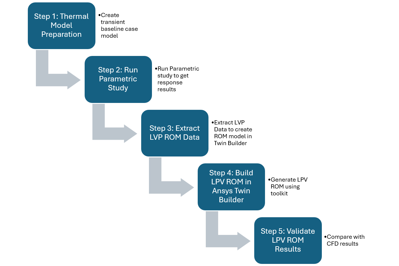
The process begins with the creation of a transient baseline model of the system. This model is then used to define a parametric study for ROM generation with the appropriate toolkits. The completed parametric runs produce response field data, which are used to build and export the ROM. The exported ROM can then be imported into Ansys Twin Builder for system-level analysis. ROM predictions should always be verified against the original CFD results to confirm that the model accurately represents the system response. Icepak supports two types of ROMs: Linear Time-Invariant (LTI) ROMs and Linear Parameter-Varying (LPV) ROMs. The differences between these ROM types are discussed in the next section.

Note: To create a steady-state ROM with spatial information, a static ROM can be created using Twin Builder; however, that approach is not covered in this blog. This blog focuses only on transient system-level ROMs using Icepak.

Linear Time-Invariant vs. Linear Parameter-Varying ROMs in Icepak

Icepak supports two types of transient system-level reduced order models depending on how the system is expected to operate: Linear Time-Invariant (LTI) ROMs and Linear Parameter-Varying (LPV) ROMs. Both are intended for system-level transient thermal prediction, where the detailed CFD model is reduced to a compact model with defined inputs and outputs.

An LTI ROM assumes that the main thermal-fluid behavior of the system remains constant during the transient simulation. In other words, the flow field, mass flow rate, and convective heat-transfer conditions are assumed to be unchanged while the power inputs vary with time. This type of ROM is appropriate when the cooling condition is fixed, such as a constant inlet velocity or a fan operating at a fixed speed. Under these assumptions, the ROM predicts the temperature response of the system for different transient power profiles without recalculating the full CFD fluid solution.

On the other hand, an LPV ROM extends the LTI approach by allowing the reduced model to vary with an operating parameter. In Icepak, LPV ROMs are particularly useful when the system behavior changes due to variations in flow rate, such as changes in the inlet velocity condition. This makes LPV ROMs more suitable for systems where both the power dissipation and the cooling condition can change over time.

It is important to note that these ROM approaches are mainly suited for forced convection applications. Natural convection can introduce additional nonlinear behavior because the flow field depends strongly on temperature-driven density changes, which may reduce the accuracy of this type of reduced order model.

This blog focuses on the creation of an LPV ROM using Icepak and Twin Builder. It assumes that an Icepak CFD model has already been created and validated. The following sections cover only the additional setup steps required to prepare the model for LPV ROM generation, with emphasis on defining the variable inlet velocity, defining the transient power inputs, setting up the parametric study using the LPV Toolkit, creating the ROM, and importing it into Twin Builder.

LPV ROM Generation Workflow in Icepak

This section discusses the requirements for creating and setting up the initial transient Icepak model. It also describes how to use the LPV ROM Toolkit to create and review the parametric setup, run the parametric analysis, and export the LPV ROM.

Create and Set Up the Icepak Transient Baseline Case

The example used in this blog is a cold plate system with three local heat sources. All the steps presented in this blog were performed in AEDT 2025 R2, but they can also be applied to other releases. The details of the cold plate used in this example are shown in Figure 2.

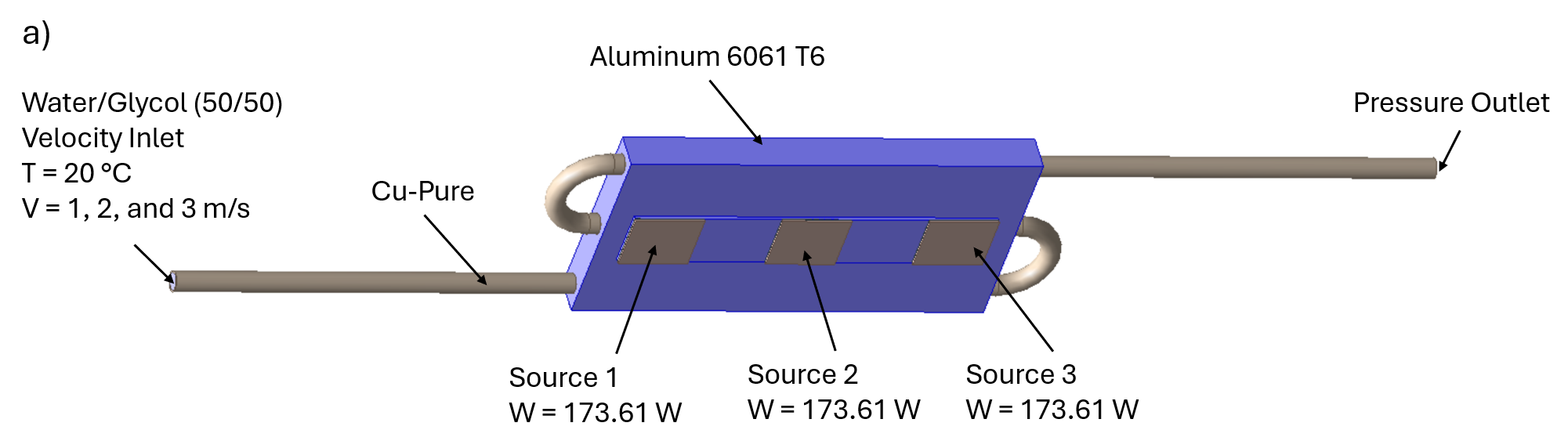
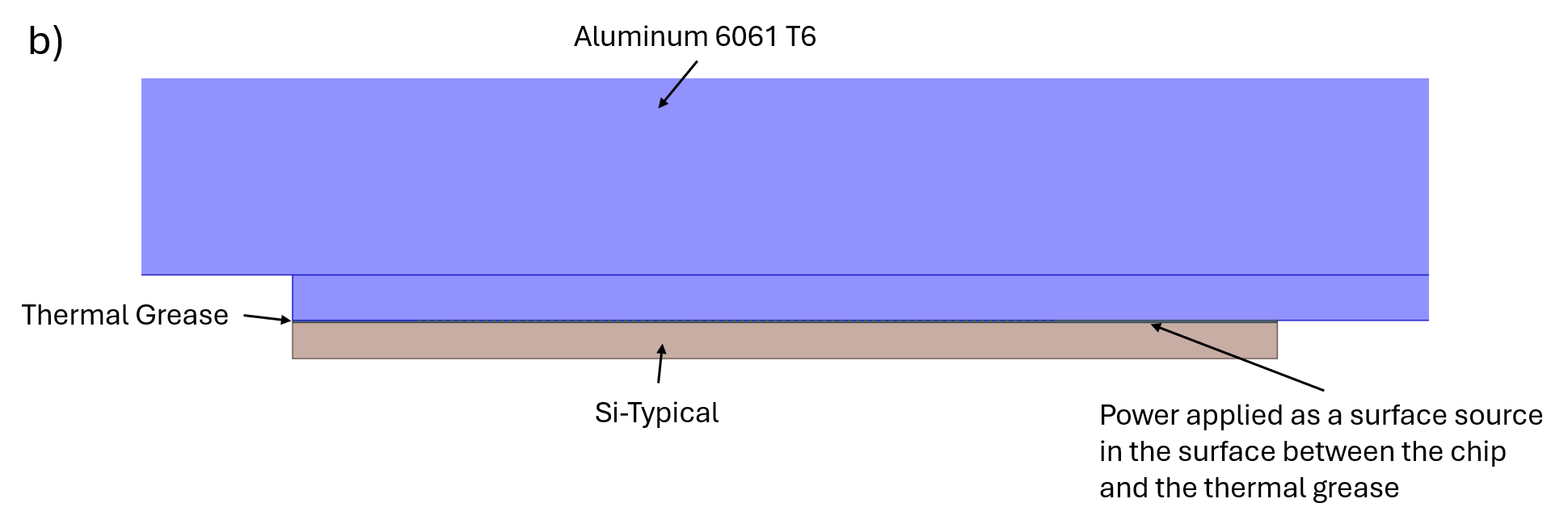
The walls surrounding the cold plate are assumed to be adiabatic, which means that heat is released only through convection with the fluid inside the cold plate. Other heat loss mechanisms, such as natural convection and radiation, are assumed to be negligible and are therefore excluded from the model. This condition is also required for the LPV model to be valid.

Create the LPV Reduced Order Model Parametric Setup

The first step in creating the LPV ROM (reduced order model) is to create the appropriate parametric setup to obtain the system response. To simplify this process, Icepak includes a specific toolkit that can be used to generate the required parametric trials. You can access this tool by clicking Icepak > Toolkit > Modeling and selecting LPV_ROM_Parametric_Setup. Note: If the solution type for your case is not set to transient, the toolkit will not work and will display an error message.

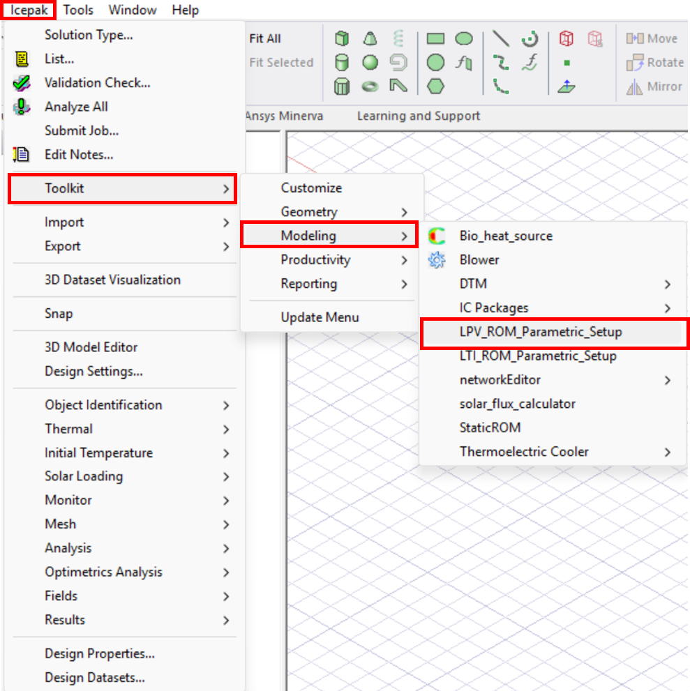
After you click LPV_ROM_Parametric_Setup, a dialog box opens. In this dialog box, you can configure which options to include in the parametric trials. The available options are explained in the list below.

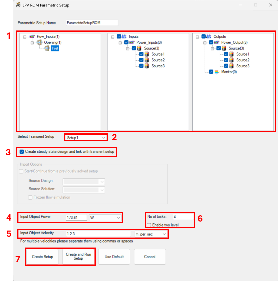
1. The toolkit automatically identifies and populates the inlet conditions and heat sources applied in your case. If you do not want to include all heat sources, you can clear the corresponding selections. For this demonstration, we will keep all of them.
2. The transient setup is also populated automatically. If you have multiple setups, you can select the correct However, it is not necessary to create multiple setups because the settings are overwritten later.
3. This option allows you to create a steady state design copy from your transient setup. The purpose of this option is to allow you to use the Frozen Flow Simulation option, if your case permits it, so you can run the steady state case for each flow condition and solve only the transient energy equation. Use this option carefully because it can create incorrect relationships between the model inputs and outputs for the ROM. For this blog, we will use this option to create a backup, but it will not be used to solve the steady state flow.
4. In the input object power box, you can assign the maximum power for your heat sources. Later in this blog, we will show that the ROM can also extrapolate results to higher heat-source values while still producing results similar to the transient CFD model.
5. In the input object velocity box, you can assign the different velocities at which you want to evaluate the system. For this case, we are using three velocities: 1, 2, and 3 m/s.
6. This option is important only if you want to run the parametric trial It manages the HPC settings. For this blog, we will skip this step because we will review the model before submitting the parametric run.
7. You can either create the setup or create the setup and run the parametric For this case, we will use the create setup option. After you click this option, the toolkit generates the LPV ROM outputs, which include the steady state setup and the transient setup with the parametric run already configured.

Understanding the LPV ROM Toolkit Output

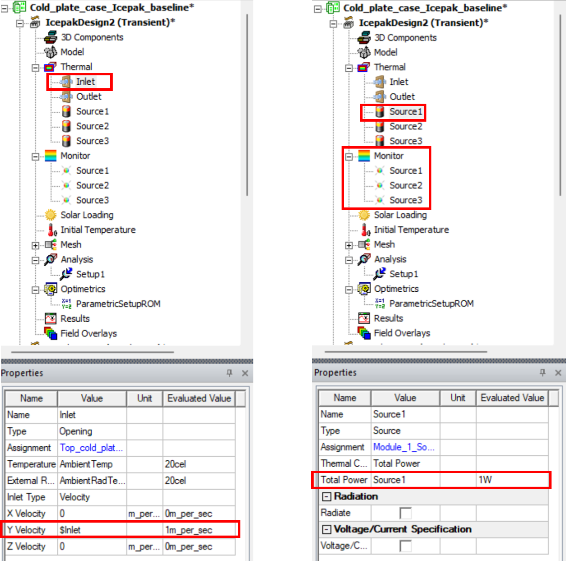
After you click Create Setup, Icepak creates a steady state copy of your case and modifies the transient setup. The first thing you may notice is that, in the new transient setup, the inlet and heat sources are assigned as variables. These variables are used by the parametric setup to execute the parametric trials. The toolkit also automatically adds monitor points for the heat sources, as shown in Figure 5.

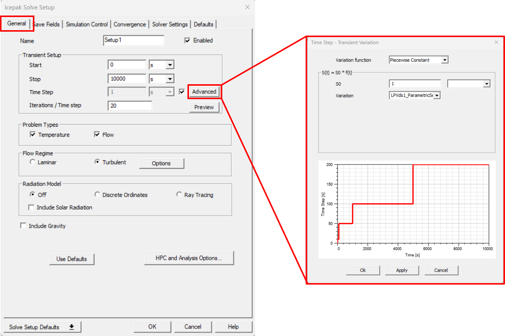
Another important change that should be double checked is the settings. Under Setup, on the General tab, you can see that the toolkit assigns a default simulation time of 10000 seconds. The time step is not constant; instead, it is defined by a piecewise constant curve, as shown in Figure 6. The purpose of this curve is to use a small time-step at the beginning of the simulation and progressively increase the time step size as time advances, so fewer steps are required later in the transient simulation. You can adjust these values according to your simulation scale and requirements. For this blog, we will use the default values.

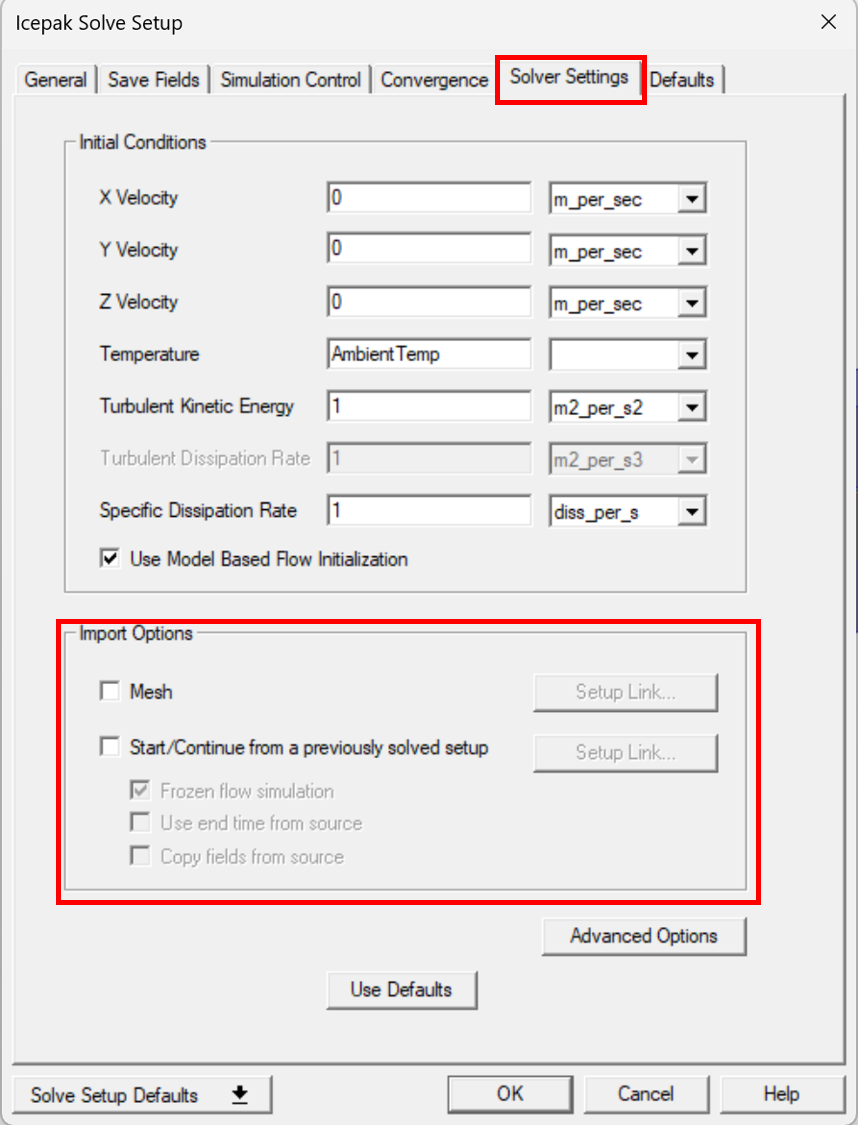
Now, in the setup configuration, on the Solver Settings tab, you can find the Start/Continue from a Previously Solved Setup > Frozen Flow Simulation option under Import Options. As mentioned earlier, use this option with caution because, depending on the case used to create the ROM, it can lead to an incorrect relationship between the input and output variables. For example, in the case used in this blog, using this option produced a ROM with an inverse relationship between sources, meaning that the temperature in source 1 was inversely proportional to the activated heat source 2 or 3, which is physically incorrect.

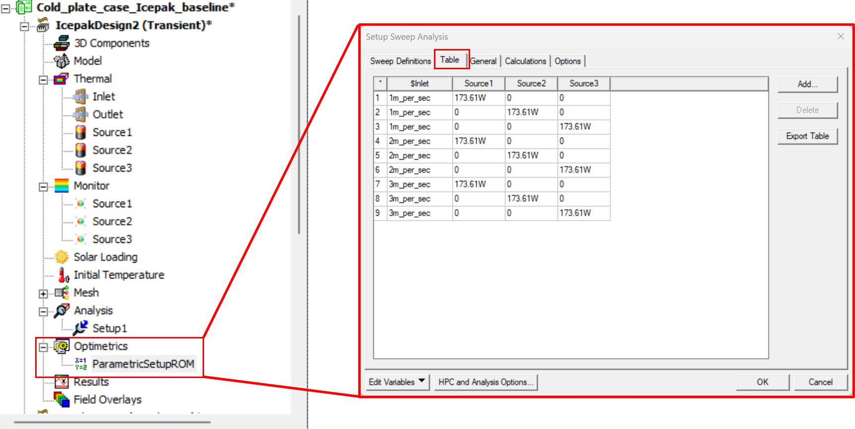
In the Project Manager, under Optimetrics, the toolkit adds the parametric setup. Double click ParametricSetupROM. In the Setup Sweep Analysis dialog box, on the Table tab, note that nine trials have been created. The LPV ROM requires the effect of each heat source to be estimated independently. For this reason, each parametric trial contains only one active heat source with a nonzero power value, while the remaining heat sources are set to zero. These independent source effects are then evaluated at the three selected inlet flow velocities to capture the influence of varying inlet conditions.

Execute the Parametric Study and Export the LPV ROM

The next step is to run the parametric setup. You can configure your HPC settings according to the licenses available to run multiple cases in parallel, or you can run them sequentially. The time required for this step will vary depending on the mesh size, transient simulation settings, total simulation time, and time step definition used for the parametric trials.

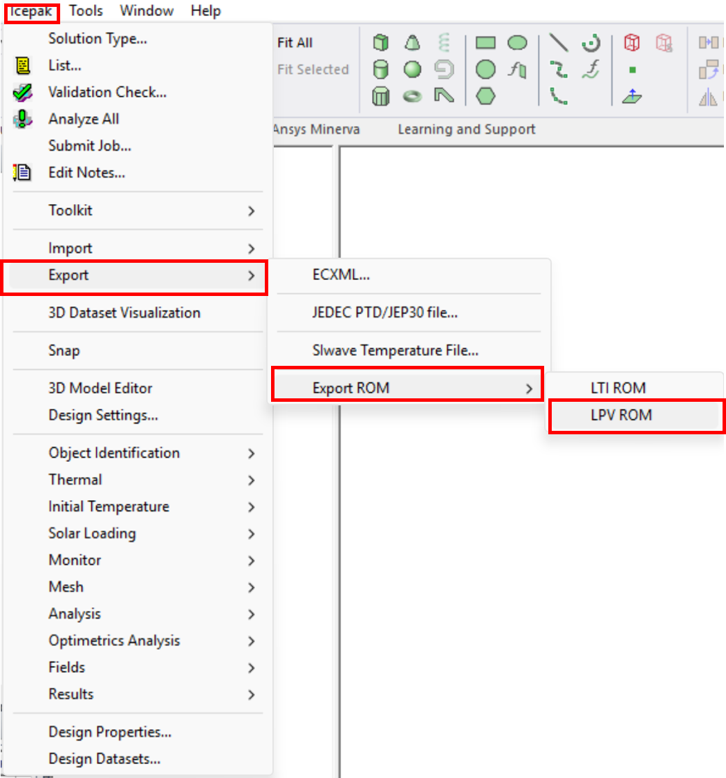
After the parametric trials have completed, the resulting solution files can be used to export the LPV ROM by selecting Icepak > Export > Export ROM > LPV ROM, as shown in Figure 9.

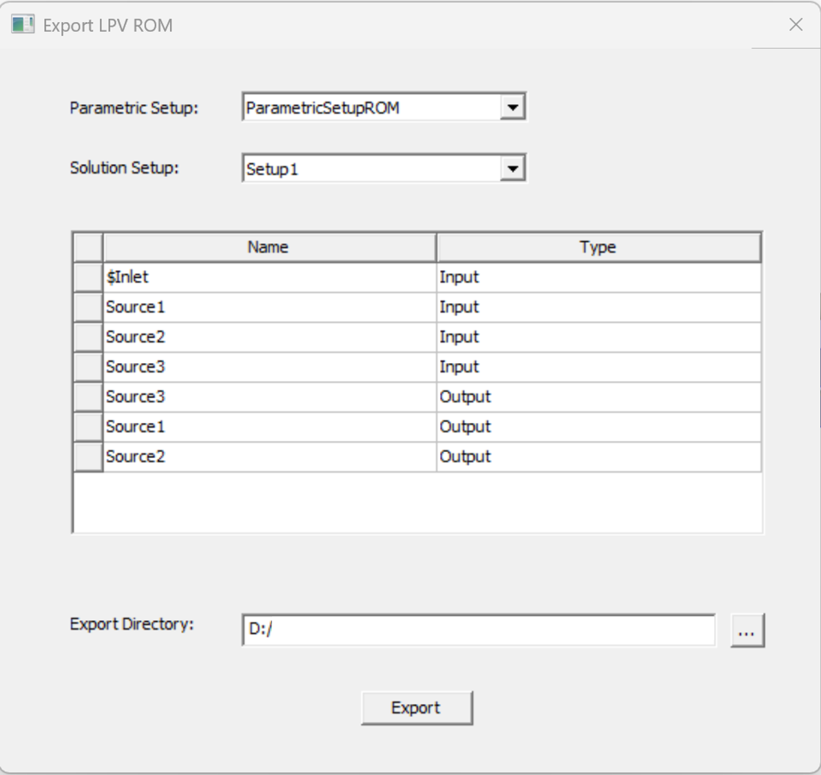
This option opens a dialog box where you can review the inputs and outputs that will be created for your reduced order model. You can also select the path where the output file will be saved. This step is important since we will need to read this folder later when we import the LPV ROM in Twin Builder.

At this stage, all the data required to import the LPV reduced order model into Twin Builder has been generated. Before the model can be used, a few additional steps are required to successfully import and create the LPV ROM in Twin Builder. The following section walks through this process.

Configuring Twin Builder and Importing the LPV Reduced Order Model

Twin Builder uses the LPV Wizard to create a Modelica ROM from the LPV ROM files exported from Icepak. Before importing the LPV ROM, a few additional Twin Builder settings must be configured to ensure that the Modelica ROM is created successfully and can be executed correctly.

Configure the Twin Builder Environment

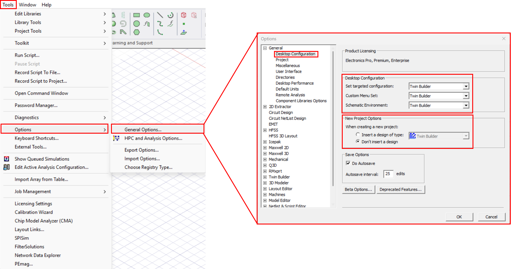
The first step is to set Twin Builder as the target configuration. To do this, go to Tools > Options > General Options. In the Options dialog box, select Desktop Configuration and set Targeted Configuration to Twin Builder. The remaining configuration settings will be updated automatically. Finally, under New Project Options, set When Creating a New Project to Don’t Insert a Design, and then click OK.

Building the LPV ROM in Twin Builder

Now that Twin Builder is set as the target configuration, the first step is to add a Twin Builder design from the Project menu.

After creating the Twin Builder design, open the LPV Wizard by selecting Twin Builder > Toolkit > LPV Wizard from the toolbar. The wizard reads the LPV ROM files exported from Icepak and uses them to generate a Modelica ROM. In the LPV Wizard dialog box, select the working directory containing the exported Icepak data. The correct folder can be identified by the _LVPROMFiles suffix in its name.

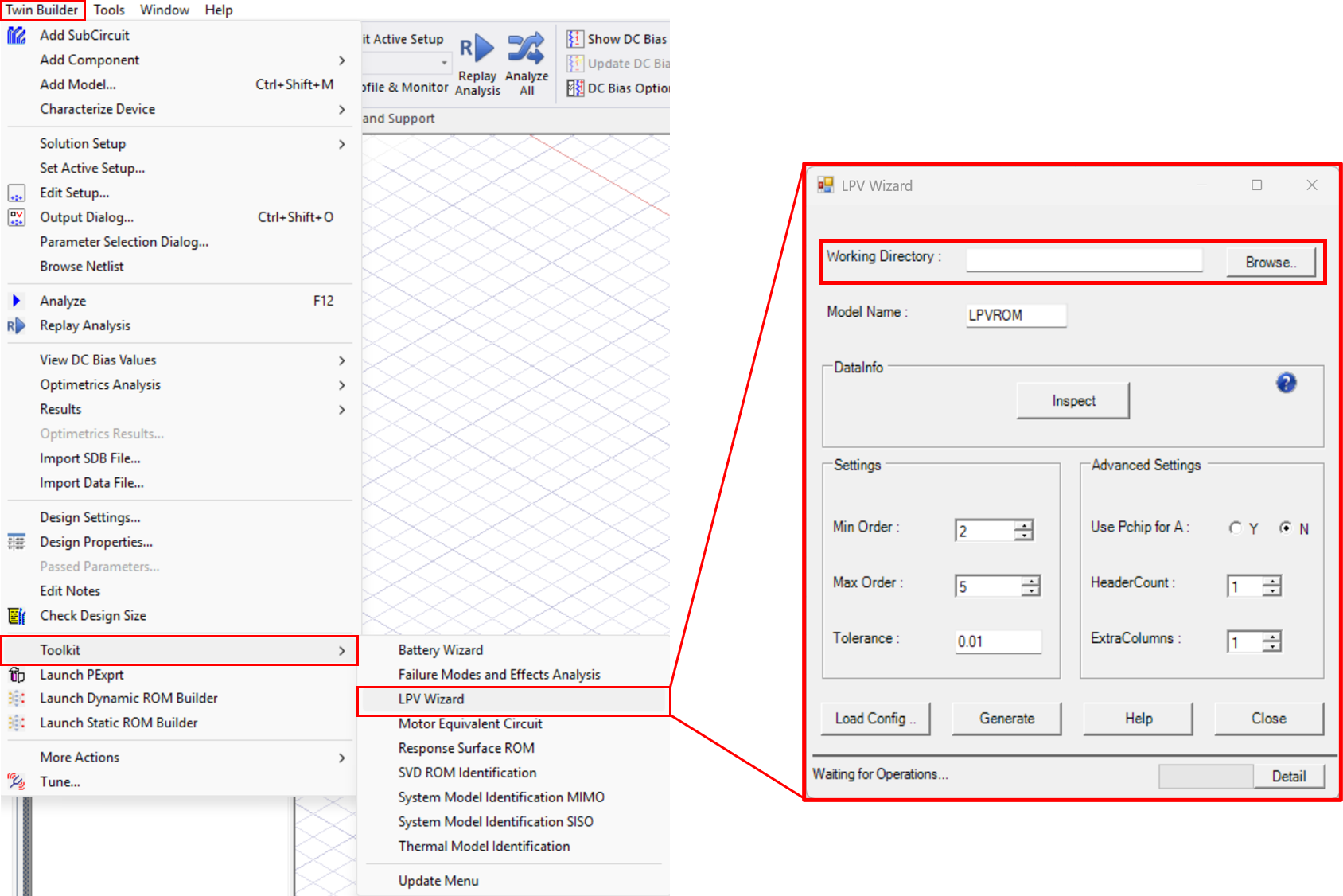
You can assign a model name and keep the default values for all other settings. Click Generate, and a pop-up window will appear indicating that the process has been completed successfully. Click OK, and then close the LPV Wizard. At this point, the Modelica ROM has been created and saved under the project’s Components directory. We are now ready to set up the ROM model in Twin Builder, compare its predictions against the transient CFD results, and validate its accuracy.

Building the Twin Builder LPV ROM Model

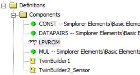
Now that the Modelica ROM has been created, we can use it in the Twin Builder model. You can find the ROM model under Definitions > Components. Select the LPVROM and drag it into the 3D modeler window. Click again to place the ROM model, and then press Esc to exit component placement mode.

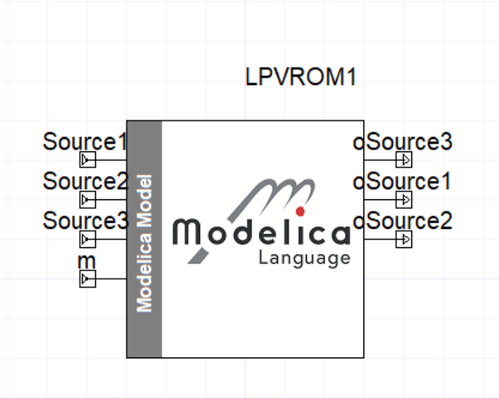
After placing the reduced order model, you will notice that the ROM is a black box with four input ports on the left and three output ports on the right. These are the inputs and outputs configured in the previous steps.

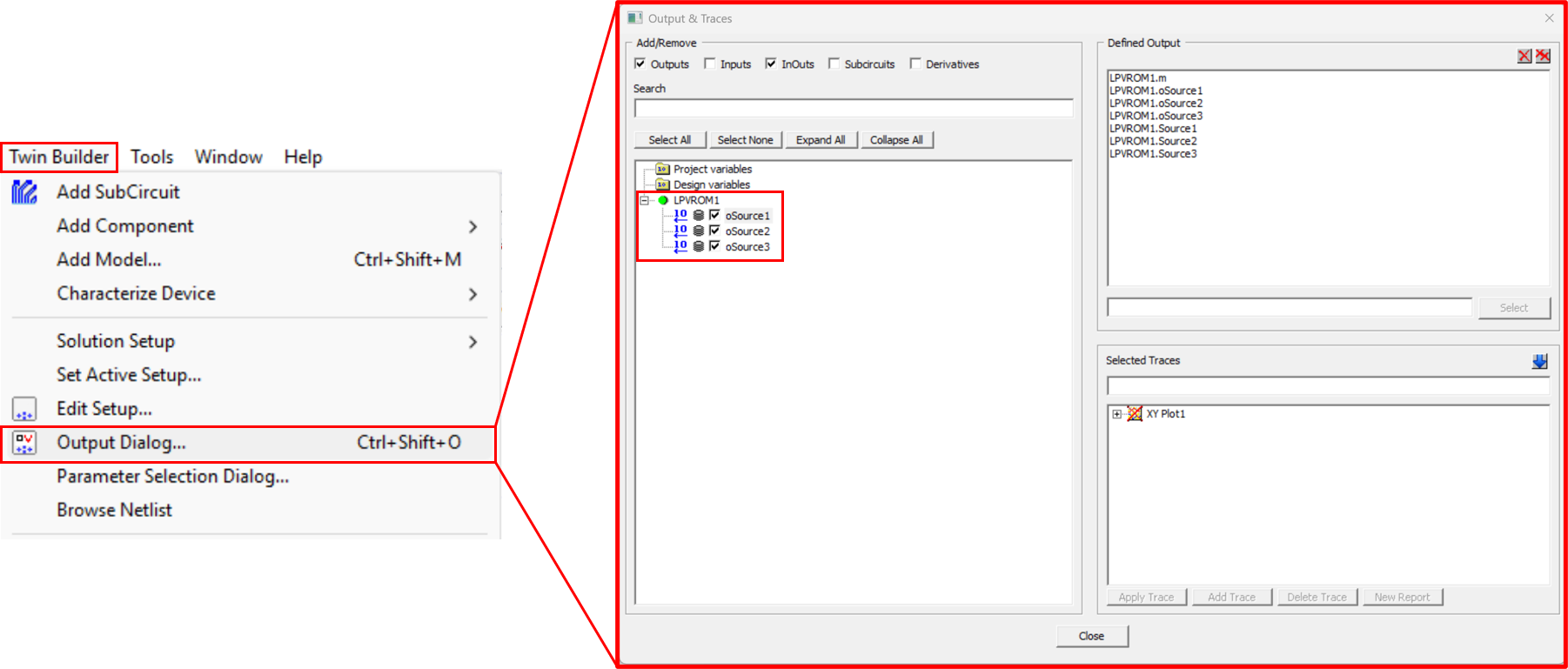
With the ROM placed, we can now configure the ROM model. The first step is to make sure the outputs are enabled. To check this, go to Twin Builder > Output Dialog and make sure the outputs are highlighted.

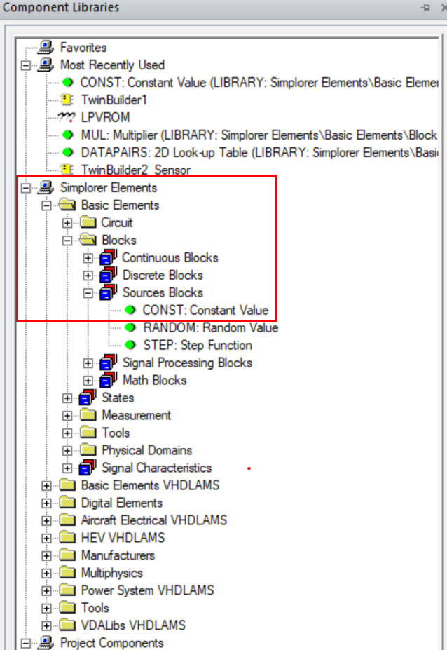
For the inputs, you can specify constant values, time-dependent values, or imported values. For this blog, we will use constant values so we can validate the results against the transient CFD model. To add a constant value block, go to Component Libraries > Simplorer Elements > Basic Elements > Blocks > Sources Blocks, and then drag CONST: Constant Value into the 3D modeler window.

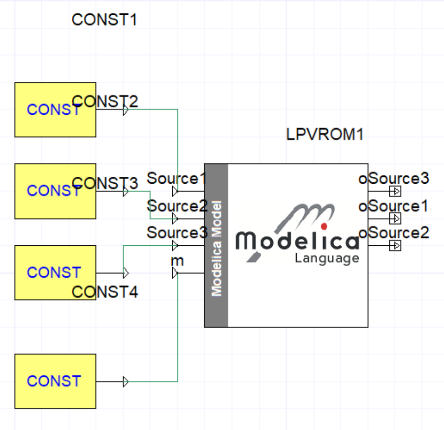
After adding a constant block for each input, the reduced order model should look like the schematic shown in Figure 18. Note: The m input corresponds to the inlet velocity.

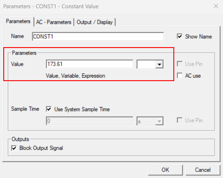
You can modify the values assigned to each constant block. When you double-click a constant block, it shows a number without units, so you need to be aware of the units used in your Icepak case when the transient files for the ROM were generated. In this example, power is defined in W and velocity is defined in m/s, so the values assigned to the constant blocks should use those units.

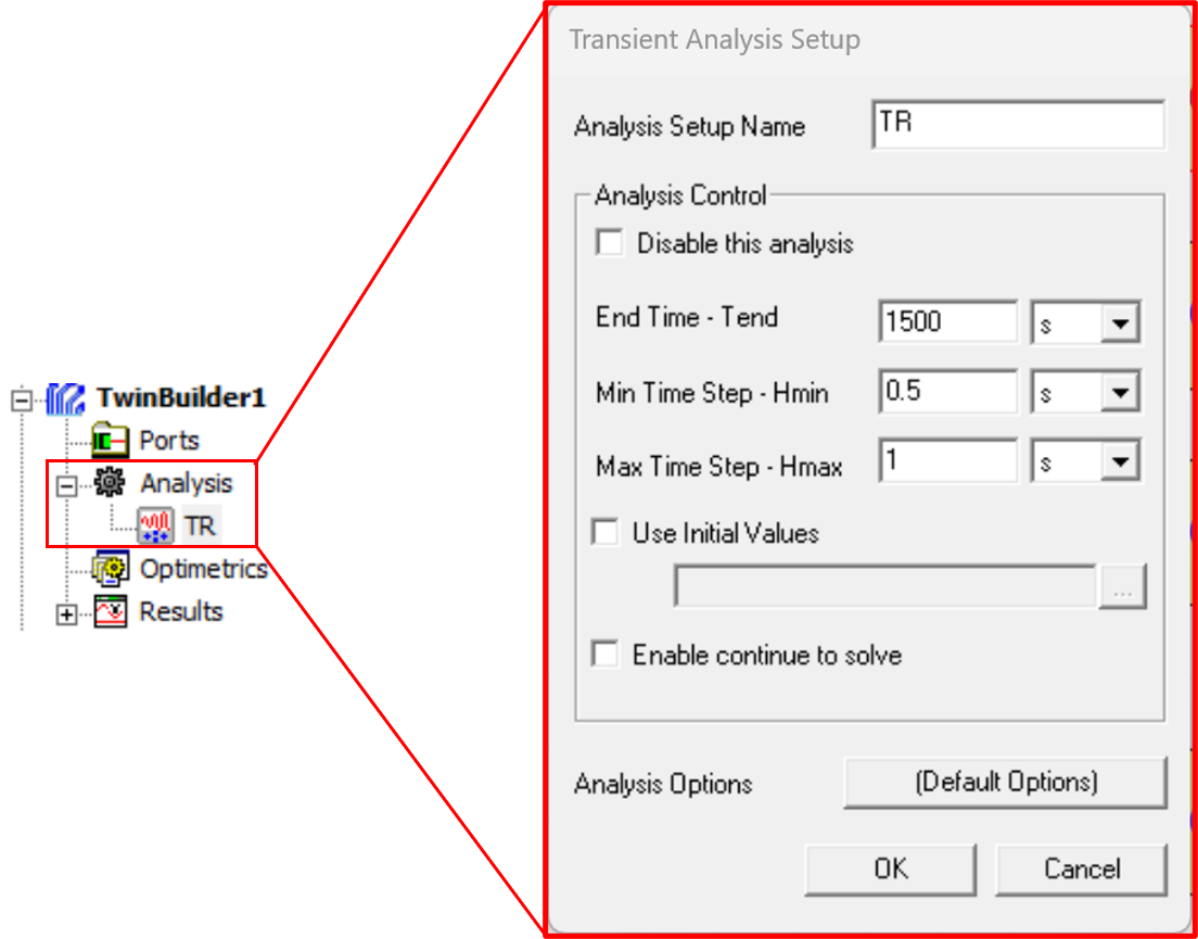
The last setup step is to configure the simulation time, including the minimum and maximum time step. You can access this option by going to Twin Builder Design > Analysis > TR. After configuring the case, right-click the setup and select Analyze.

Postprocessing Reduced Order Model (ROM) Results

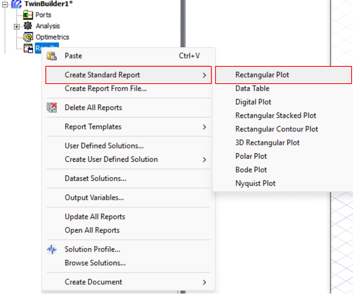
After a few seconds or minutes, the LPV ROM model will solve. The next step is to postprocess the results. First, we can plot the time-dependent results for the three different sources. To do this, under the Twin Builder design, right-click Results and select Create Standard Report > Rectangular Plot.

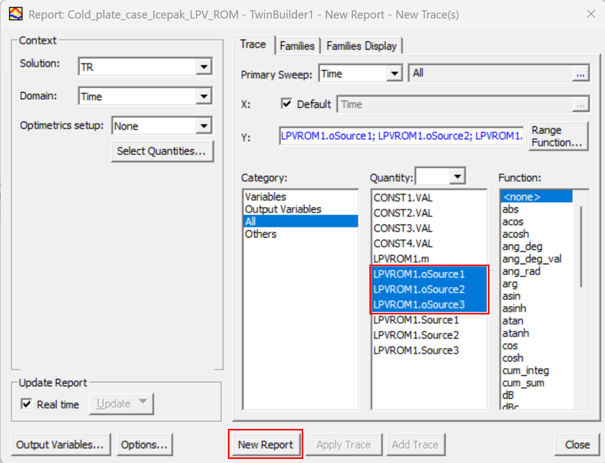
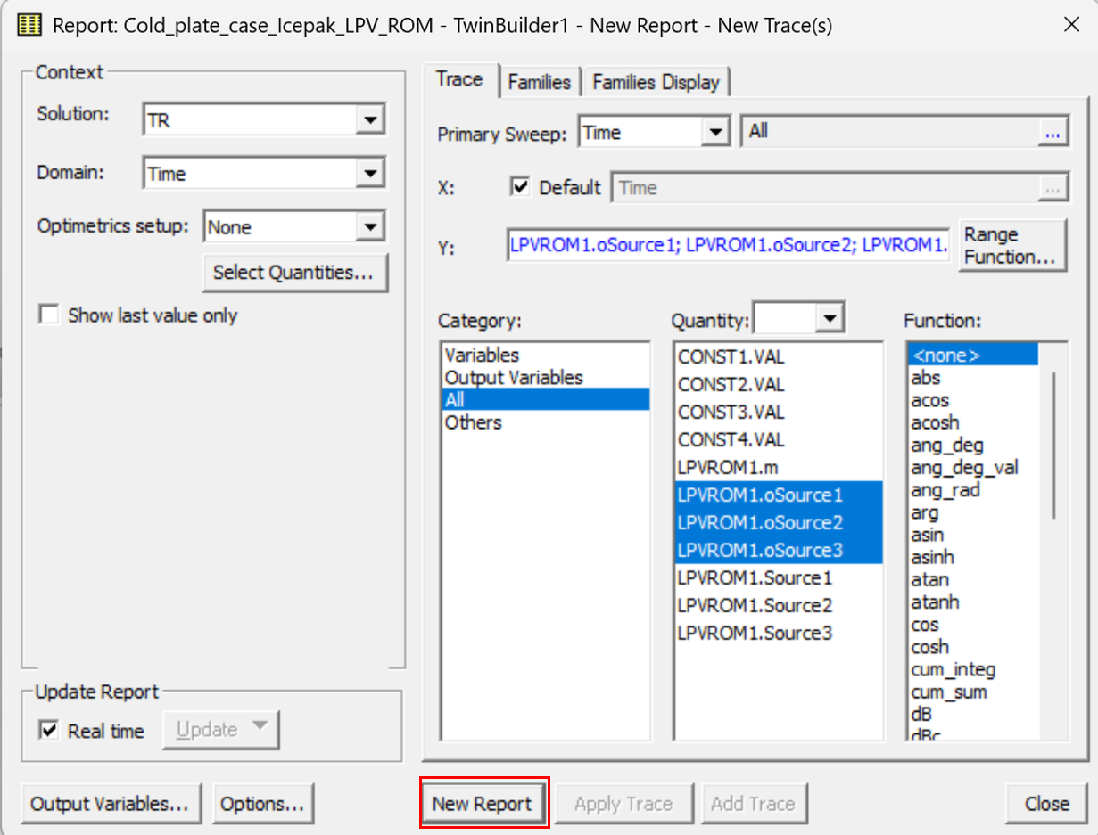
This option opens a dialog box where you can select the output variables to plot. In this case, we selected the ROM output variables for each source. Then click New Report.

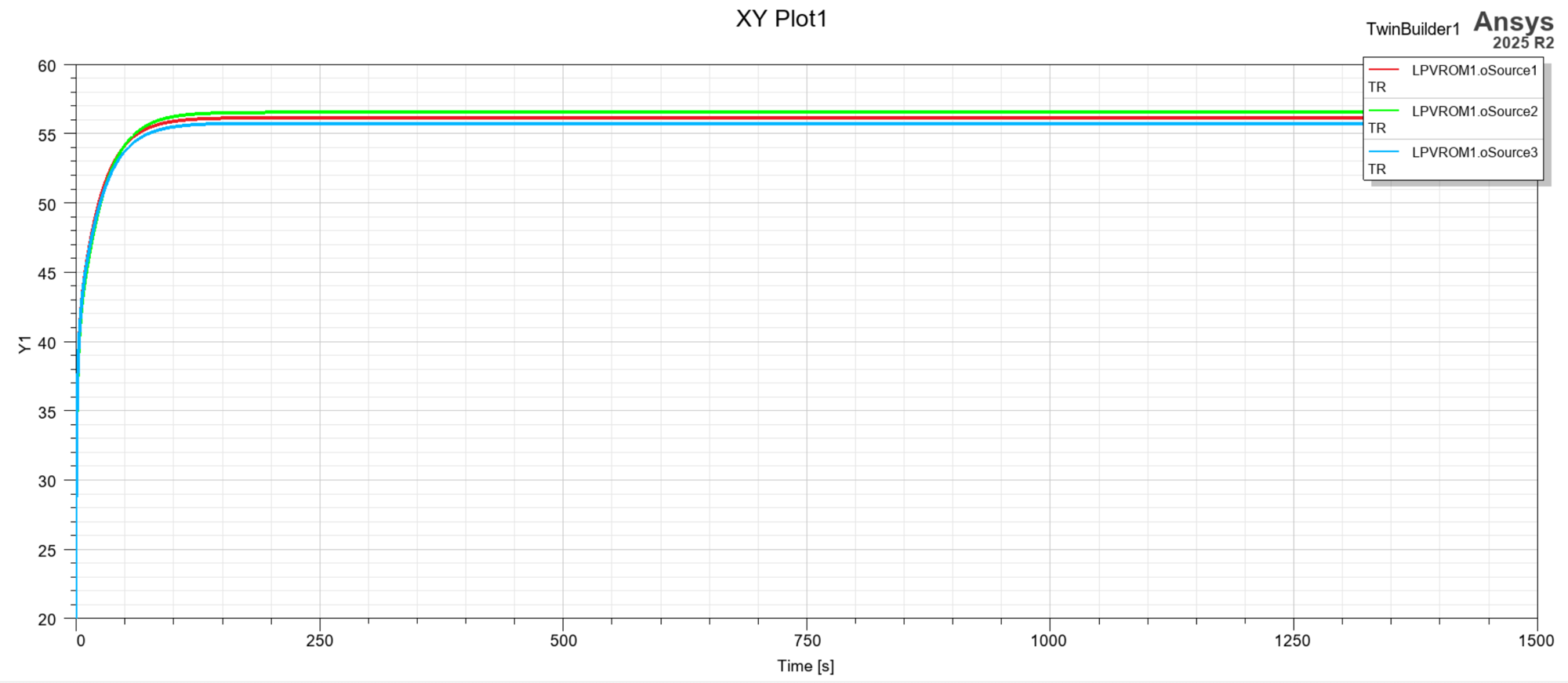
The figure you create using this option is shown in Figure 23.

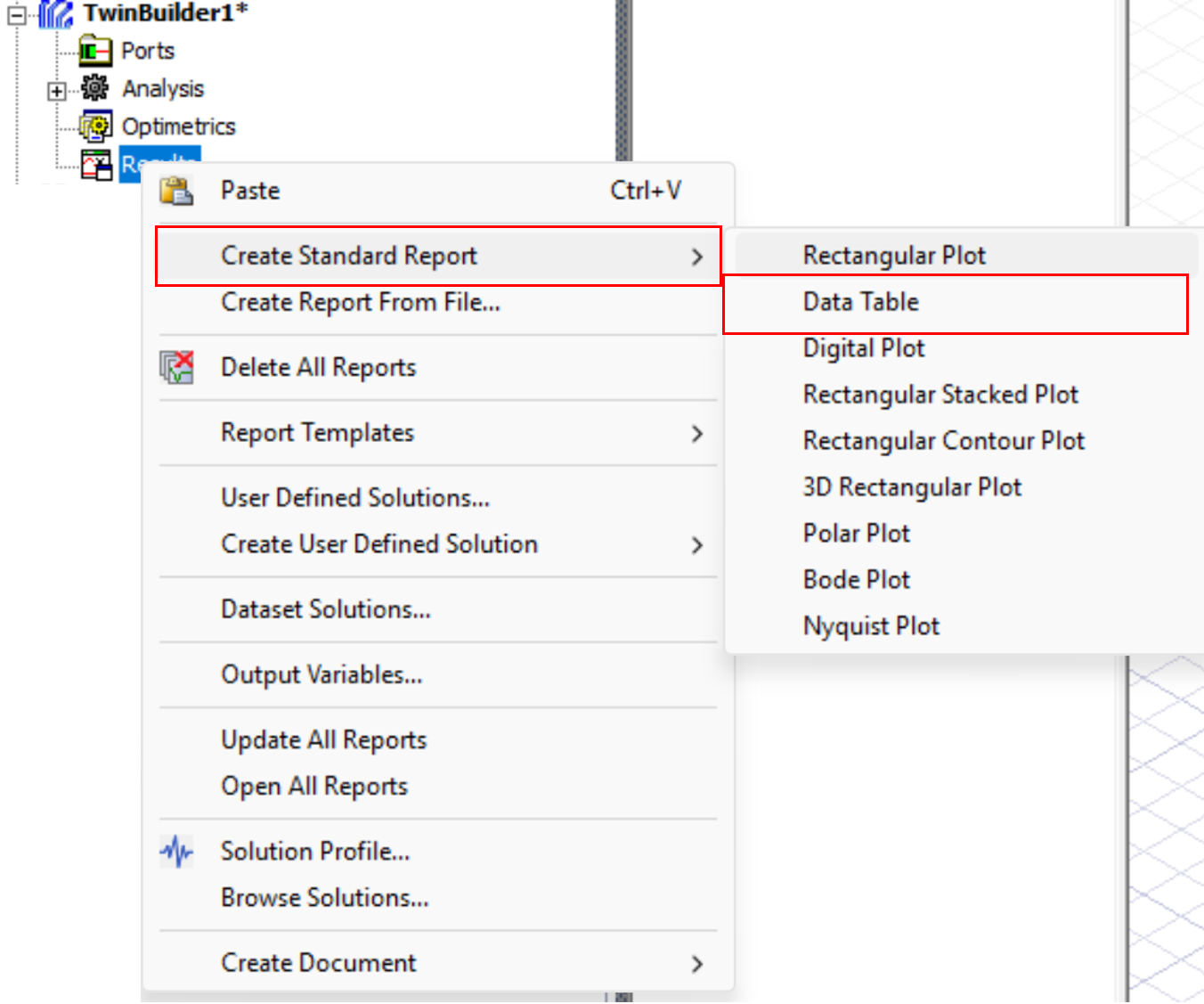
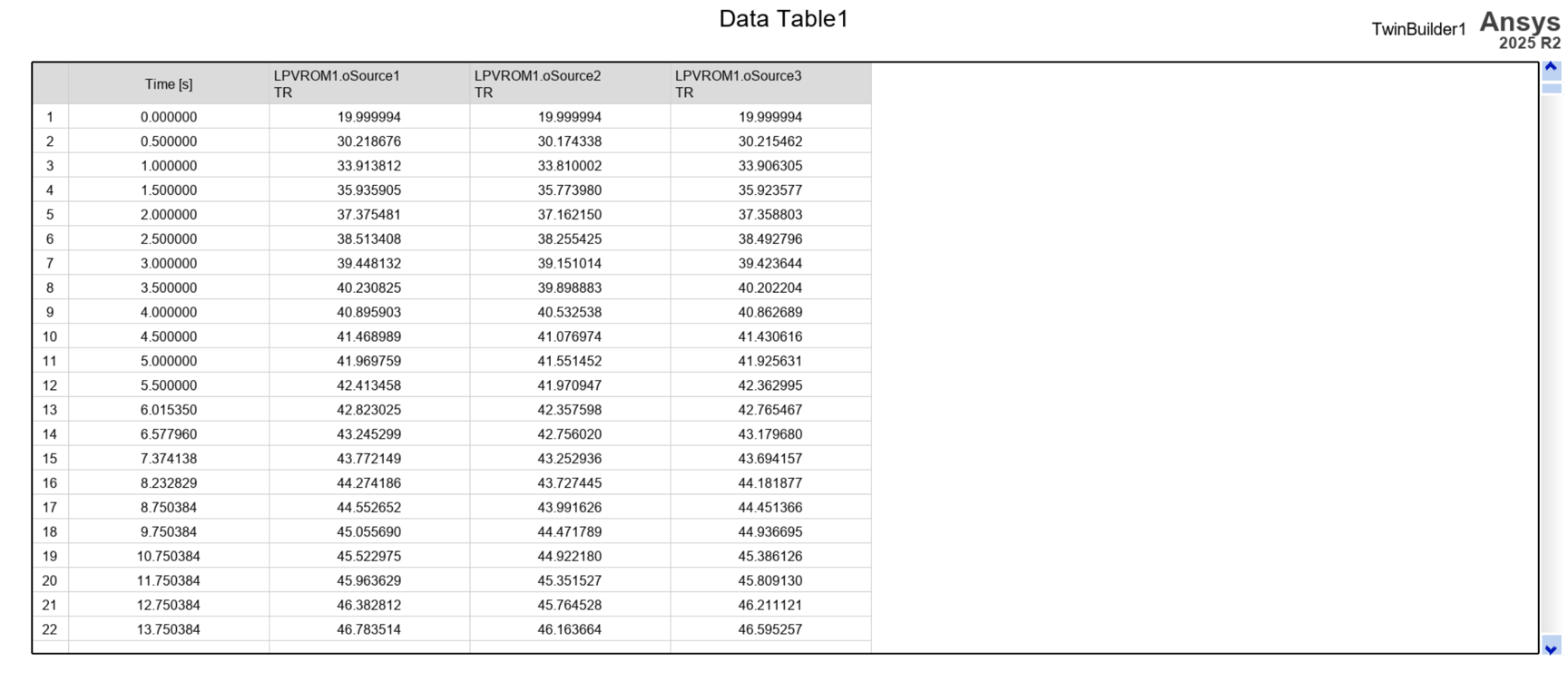
Another option is to create an output table with the results so you can export it later for further postprocessing. To do this, under the Twin Builder design, right-click Results and select Create Standard Report > Data Table.

As before, this option opens a dialog box where you can select the output variables to include in the table. In this case, we selected the reduced order model output variables for each source. Then click New Report.

The data table created using this option is shown in Figure 26. You can right-click the table and export it in .csv format for further postprocessing. This was the procedure used for the results shown in the next section of this blog.

Validating Reduced Order Model Results and Comparing Them with Transient CFD Results

For the ROM created in this blog, seven cases were compared against the transient CFD results to evaluate the accuracy of the reduced order model. The list of tested cases is shown in the table below.

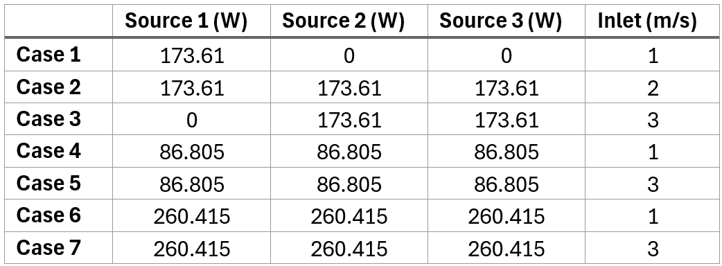
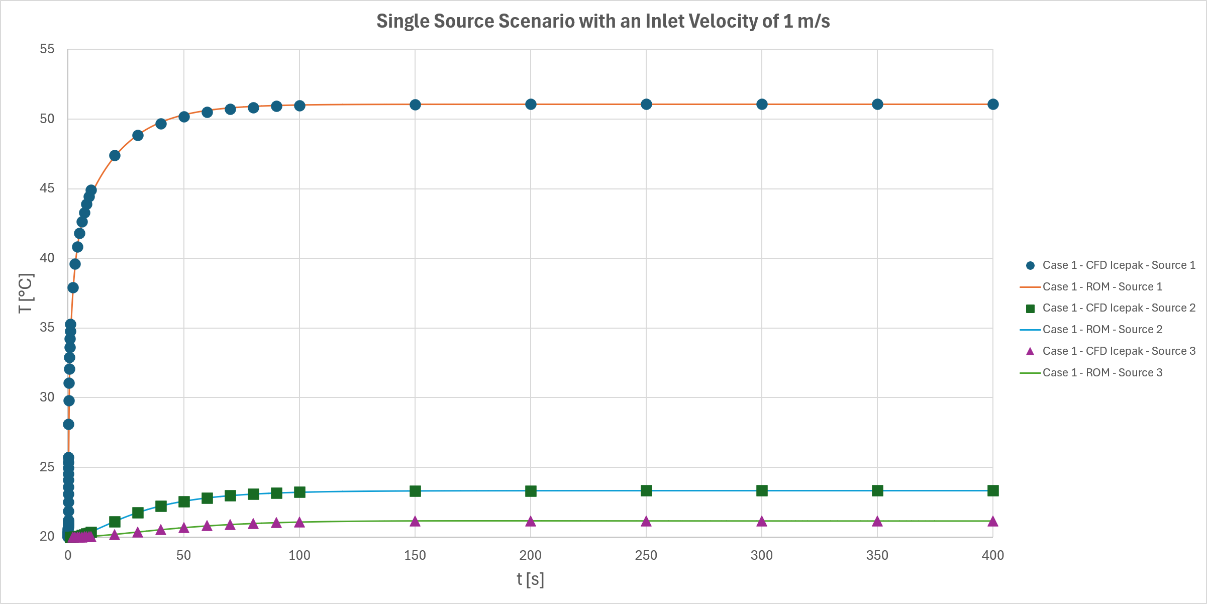
Figure 27 shows the comparison between the ROM results for the three sources and the transient CFD results. The results show good agreement; however, it is worth mentioning that this transient case was one of the cases used to create the ROM.

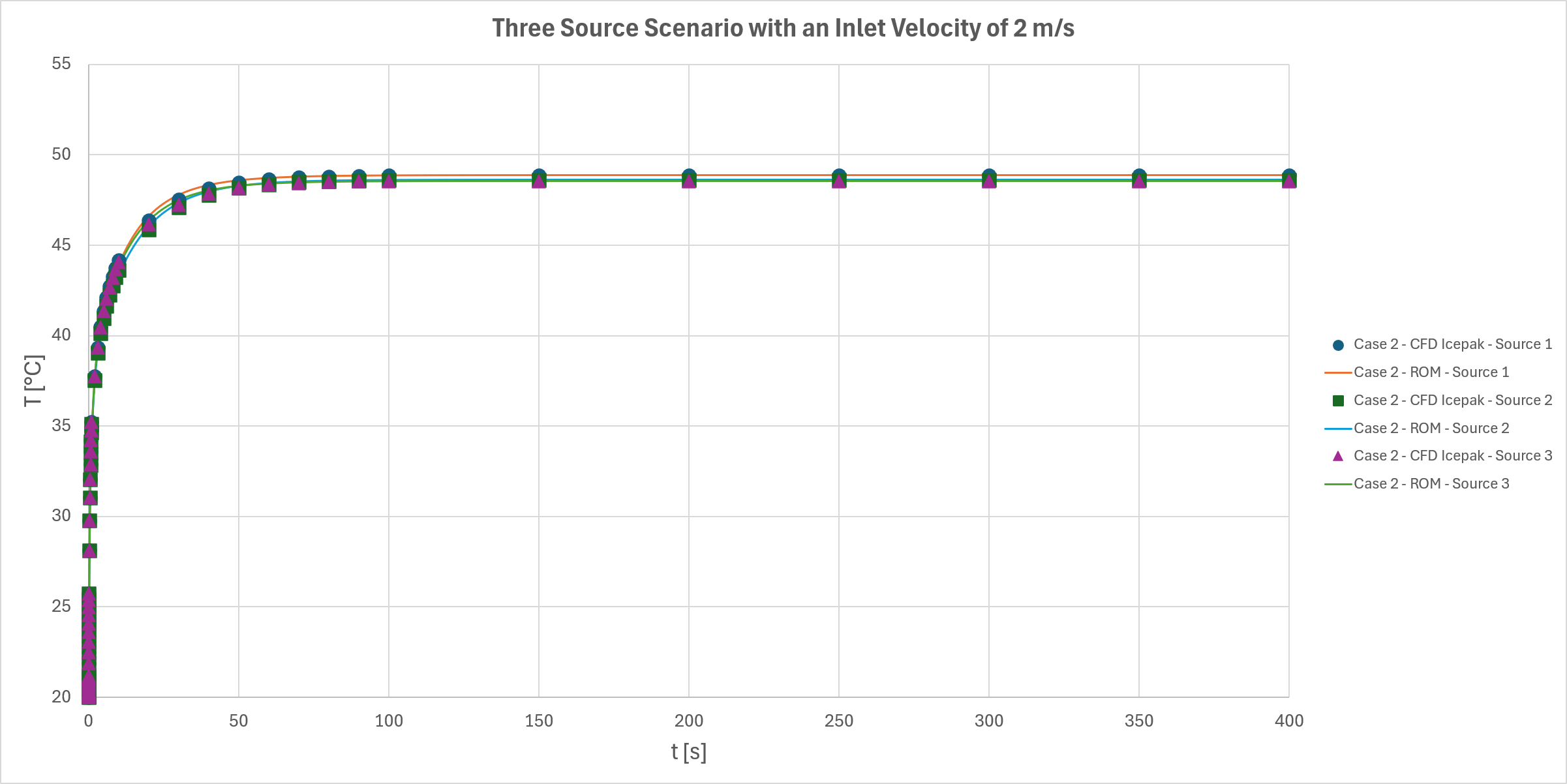
When testing configurations that were not used to create the ROM, such as the three sources at 173.61 W with an inlet velocity of 2 m/s, the results show good agreement as well, between the ROM prediction and the CFD results. We can also see that the ROM accurately predicts the steady-state solution, although there are some discrepancies during the first 100 s.

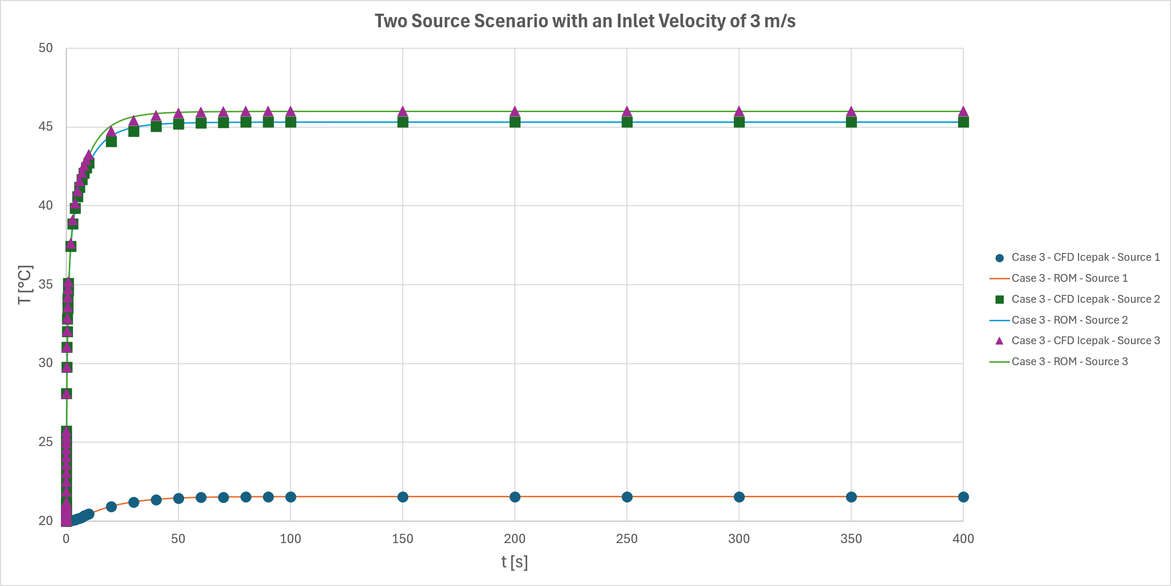
Furthermore, we also compared the solution with a two-source scenario. In this case, the steady-state solution is almost the same, but some discrepancy remains during the first 100 s.

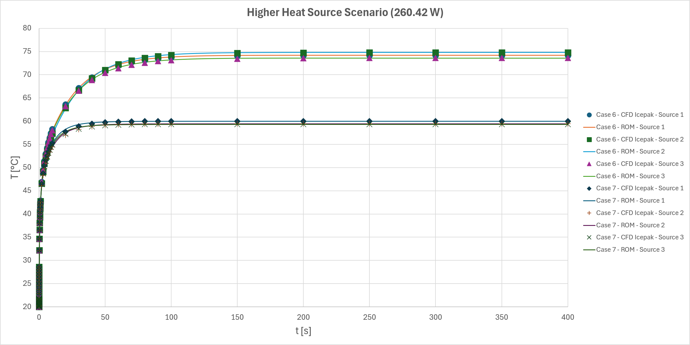
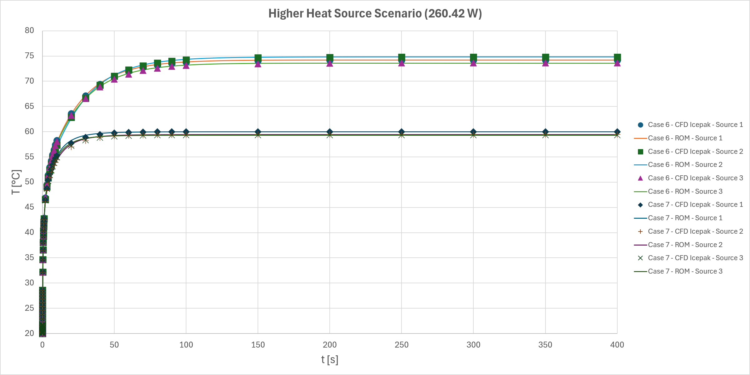
Initially, you might think that this model is accurate only when the source values are lower than the training value. However, testing shows that the reduced order model is accurate for lower source values and can also provide meaningful, accurate results when the heat source power is increased, as shown in Figure 30 and Figure 31, even for different inlet conditions.

In general, this comparison shows the capability of the ROM model to provide accurate transient results in a matter of minutes. This allows us to test different boundary conditions and variable inputs, and to analyze the system-level response more efficiently.

Reduced Order Model Conclusions

Reduced order models provide an efficient way to extend detailed Icepak CFD results into fast system-level thermal simulations. In this blog, we walked through the process of creating an LPV ROM for an electronics cooling application, starting from a transient Icepak baseline model, generating the required parametric trials, exporting the ROM data, and importing the model into Twin Builder. This workflow allows engineers to preserve the main transient thermal behavior of the original CFD model while significantly reducing simulation time, making it practical to evaluate different power levels, inlet velocities, and operating scenarios.

The validation cases showed that the LPV ROM can provide good agreement with transient CFD results, especially for steady-state temperature predictions and overall transient trends. Some differences may appear during the early transient response, so it is important to validate the ROM against representative CFD cases before using it for broader system studies. Once validated, the LPV ROM becomes a valuable tool for design exploration, digital twin workflows, and system-level thermal analysis where fast turnaround time is critical.

Ansys Solution Benefits

Ansys provides powerful thermal simulation capabilities for semiconductor design, enabling engineers to analyze geometry configurations, material properties, interconnect types, or cooling technics—all without building physical prototypes. Ansys has specialized tools like Icepak for electronics cooling, SiWave for signal and power integrity, Maxwell and HFSS for electromagnetic analysis, Mechanical for structural and thermal simulations, Ansys Fluent for thermal and fluid simulations, and DesignXplorer and OptiSLang for design optimization and parametric evaluation, making it a comprehensive suite for multi-physics modeling and performance refinement.

Need help building reduced order models for electronics cooling with Ansys Icepak and Twin Builder? Connect with SimuTech Group to discuss your simulation goals.

Additional Reading

Twin Builder CFD Example: Building, Validating, and Evaluating a Static ROM

Singular Value Decomposition Reduced Order Model for Battery Module

Creating a Reduced Order Model for Vortex Prediction in a Stirred Tank

LTI Reduced Order Models for Battery Module Thermal Simulation in Ansys Fluent and Twin Builder