Time-Transient Thermal Analysis in Ansys FEA
When performing a time-transient thermal analysis in FEA, it is common to have bulk temperature loads and convective heat transfer coefficients that change values during the transient. Consider the example of both water temperature and flow rate in a pressure vessel changing over time.
The bulk temperature of the water may change at times that differ from times at which the flow rate changes. Bulk temperature may ramp up and down slowly, whereas water flow rates may change quickly as pumps go on or off, or as valve positions change.
Describing Time-Dependent Values as Functions
In thermal transient analysis, time-dependent values of the bulk temperature and convection coefficients must be described as functions of time within the corresponding Thermal Software. In the Ansys finite element analysis program, Table Arrays are often employed to describe these time-dependent functions. This “tips & tricks” article presents a simple example of such a procedure.

Analyzing Time-Varying Loads in Ansys
Ansys can form solutions at a variety of times during a transient analysis. Major load changes can be formed at the ends of individual load steps, with a SOLVE command executed for each load step. Loads can be step-changed from one load step to another if the command KBC,1 is executed prior to SOLVE.
Ansys KBC Settings for Loading
The default KBC,0 setting ramps loads from one load step to another. In transient or nonlinear analysis, it is usually important to form intermediate time solutions inside load steps, at several substeps. It is common to guide the number of substeps with a DELTIM command in transient analysis, or a NSUBST command in static nonlinear analysis.
The default KBC,0 setting causes loads during the substeps to ramp up or down in value from one load step to another. The KBC,1 setting will cause loads to instantly change value to the final setting for the load step, from the first substep onward. As mentioned above, a convective heat transfer coefficient may have a nearly instantaneous step change, while a bulk temperature may change with a much slower ramped value.
Calculating with Load Volatility in Mind
There are two commonly used ways in Ansys in which a blend of suddenly changed loads can be mixed with loads that ramp up and down gradually.
- A short time interval load step can be employed in which a load of interest ramps up, changing value quickly. In a longer load step that follows, another load can ramp up gradually over a long-time interval. Multiple load steps will be used to employ this technique.
- Alternatively, a single load step is employed, while the loads are described in time-dependent Table Array entries. Solutions are formed at all times entered in the time-dependent Table Arrays, and at other substeps. This technique can be seen inside Workbench Mechanical models that have time-varying loads.
The purpose of this document is to illustrate the time-dependent Table Array technique for describing time-dependent loading when using the Ansys Mechanical APDL finite element analysis program, with a blend of rapidly-changing loads and slowly-changing loads in the model, as often seen in thermal transient work.
Ansys Thermal Modeling | Practical Example
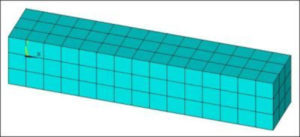
A simple Ansys thermal model is built with 8-node brick SOLID70 thermal elements. A solid bar is formed, and map meshed. The only load on this model will be a time-varying convection load on one end. The following APDL commands build the model. Note required material values Density, Thermal Conductivity, and Specific Heat:
! Example Thermal Transient Analysis\
! Units inches-seconds-BTU
!
! Convection loads with independently varying
! convection coeff and bulk temperature
!
fini
/clear,nostart
!
/PREP7
!
! Material properties– 1020 steel
MP,EX,1,30023280.0
MP,NUXY,1,0.290000000
MP,ALPX,1,8.388888889E-06
MP,DENS,1,7.346344000E-04
MP,KXX,1,6.252196000E-04
MP,C,1,38.6334760
!
ET,1,SOLID70
BLOCK,0,5,0,1,0,1 ! Block 5x1x1 inches in size
LESIZE,all,1/3,,,,,,,1
!
MSHAPE,0,3D
MSHKEY,1
vmesh,1
/VIEW,1,1,2,3
/ANG,1
eplot
FINISH
A simple block of SOLID70 thermal elements is formed:
Ansys Thermal Loading Log
A thermal transient analysis is planned for the above model. The following commands set up the transient analysis:
/SOLU
ANTYPE,4 ! transient analysis
TRNOPT,FULL ! full transient analysis
KBC,0 ! ramp loads up and down
!
! Time stepping
TIME,1000 ! end time for load step
AUTOTS,ON ! use automatic time stepping
DELTIM,10,2,50 ! substep size (seconds)
! — minimum value shorter than smallest
! time change in the table arrays below
Note the solution time commands in the above code fragment. The final TIME is set to 1000 seconds. Time substep size is permitted to range from a minimum of 2 seconds to a maximum of 50 seconds in the DELTIM command. A first substep of 10 seconds is applied. Automatic time substep sizing will vary substeps between the extremes.
A Table Array is used for the time-dependent Convection Coefficient values. Times go in the Zeroth column, while associated Convection Coefficients go in the First column. A hard copy X-Y figure of the table is plotted at the end:
! Time-dependent convection coefficient in a Table Array
! Declare Table Array — 6 times, 1 column, 1 row, Zero_th column name TIME
! Convection coefficient as a function of TIME
!
*DIM,my_conv,table,6,1,1,TIME ! 6 rows, One Column, function of time
!
! Zero out the “zeroth” row values for neatness
my_conv(0,1)=0.0
!
! Enter the times in the “zeroth” column
my_conv(1,0)= 0 ! start time
my_conv(2,0)= 120 ! end of first “flat” zone
my_conv(3,0)= 130 ! ramps up in 10 seconds
my_conv(4,0)= 700 ! end of second “flat zone
my_conv(5,0)= 710 ! ramps down in 10 seconds
my_conv(6,0)=1000 ! end of third “flat” zone
!
! Enter convection coefficients at above convection times
my_conv(1,1)=0.0001 ! Convection coefficient at start
my_conv(2,1)=0.0001 ! Convection coefficient constant, first 120 seconds
my_conv(3,1)=0.0005 ! Convection coefficient ramped up in 10 seconds
my_conv(4,1)=0.0005 ! Convection coefficient at time=700 seconds
my_conv(5,1)=0.0002 ! Convection coefficient ramped down in 10 seconds
my_conv(6,1)=0.0002 ! Convection coefficient constant, last 290 seconds
! X-Y plot Convection Coeff vs Time
/title,Convection Coefficient versus Time
*VPLOT,my_conv(1,0),my_conv(1,1)
! Hard copy of plot in working directory
/ui,copy,save,png,graph,color,norm,portrait,yes
The X-Y plot of the Table Array contents can be used to check that the numbers entered are reasonable—it is easy to put a decimal point in the wrong location. Such plots might be included in the appendices of a report:
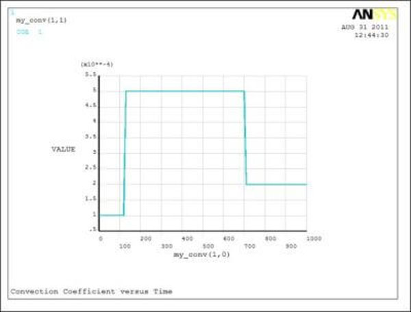
Note the sudden changes of convection coefficient in the above plot. As can be seen in the Table Array contents in the code fragment above, the coefficient has changed in 10 seconds. A physically realistic time interval needs to be employed by the user. Too short an interval can cause a non-physical response by the FEA model.
IMPORTANT: The minimum time interval in the DELTIM command must be shorter than the smallest time interval for any Table Array that describes time-dependent loading, with Time entries in the Zeroth column.
A second Table Array is used to describe the time-dependent fluid Bulk Temperature for the heat transfer convective loading. If the same times were used as in the Convection Coefficient, then the entry could be in a Second column of the Table Array used for the Convection Coefficient. In this example, some of the times at which Bulk Temperatures change will differ from times at which Convection Coefficients change, so an independent Table Array will be employed:
! Time-dependent bulk temperature in a Table Array
! Declare the array — 6 times, 1 column, 1 row, Zero_th column name TIME
! Convection coefficient as a function of TIME
!
*DIM,my_bulk,table,6,1,1,TIME ! 6 rows, One Column, function of time
!
! Zero out the “zeroth” row values for neatness
my_bulk(0,1)=0.0
!
! Enter the times in the “zeroth” column
my_bulk(1,0)= 0 ! start time
my_bulk(2,0)= 120 ! end of first “flat” zone
my_bulk(3,0)= 500 ! temperature ramps up in 380 seconds
my_bulk(4,0)= 700 ! hold temperature constant for 200 seconds
my_bulk(5,0)= 900 ! temperature ramps down in 200 seconds
my_bulk(6,0)=1000 ! end of second flat zone
!
! Enter bulk temperatures at above bulk temperature times
my_bulk(1,1)=100 ! bulk temperature at start
my_bulk(2,1)=100 ! bulk temperature constant for 120 seconds
my_bulk(3,1)=300 ! bulk temperature ramps up in 380 seconds
my_bulk(4,1)=300 ! bulk temperature constant for 200 seconds
my_bulk(5,1)= 75 ! bulk temperature ramps down in 200 seconds
my_bulk(6,1)= 75 ! bulk temperature constant, last 100 seconds
! Form a numerical Array for times for TSRES commands
! Solutions will be formed at these times, plus others
! Use ALL the times in both the “my_conv” and “my_bulk” Table Arrays
! The ZERO time is not required
!
*dim,myTSRES,array,7 ! Dimension a numerical Array, 7 rows, 1 column
!
myTSRES(1)= 120 ! as found in both arrays
myTSRES(2)= 130 ! as found in my_conv array
myTSRES(3)= 500 ! as found in my_bulk array
myTSRES(4)= 700 ! as found in both arrays
myTSRES(5)= 710 ! as found in my_conv array
myTSRES(6)= 900 ! as found in my_bulk array
myTSRES(7)=1000 ! as found in both arrays
!
! X-Y plot Bulk Temperature vs Time
/title,Bulk Temperature versus Time
*VPLOT,my_bulk(1,0),my_bulk(1,1)
! Hard copy of plot in working directory
/ui,copy,save,png,graph,color,norm,portrait,yes
Note that the Table Array times differ from those used in the Convection Coefficient table.
Charting Bulk Temperature Variation over Time in Ansys
The *VPLOT command is again used to generate a plot of the Table Array contents. A view of the plan for Bulk Temperature variation over time is seen:
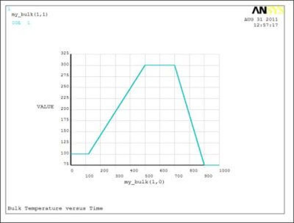
As mentioned, the Bulk Temperature is varying more slowly than the Convection Coefficient, sometimes at different Time points.
Transient Thermal SOLVE
This model is to be solved in one-time step. For this reason, a TSRES command is used for forcing the solver to include a SOLVE at every time point in the two Table Arrays above. This ensures that the time-dependent curves are followed by the transient analysis. Intermediate solutions between the TSRES time points will be included according to the DELTIM command and the automatic time stepping decisions of the Ansys solver:
! Form a numerical Array for times for TSRES commands
! Solutions will be formed at these times, plus others per DELTIM and AUTOTS
! Use ALL the times in both the “my_conv” and “my_bulk” Table Arrays
! The ZERO time is not required
!
*dim,myTSRES,array,7 ! Dimension a numerical Array, 7 rows, 1 column
myTSRES(1)= 120 ! as found in both arrays
myTSRES(2)= 130 ! as found in my_conv array
myTSRES(3)= 500 ! as found in my_bulk array
myTSRES(4)= 700 ! as found in both arrays
myTSRES(5)= 710 ! as found in my_conv array
myTSRES(6)= 900 ! as found in my_bulk array
myTSRES(7)=1000 ! as found in both arrays
!
TSRES,%myTSRES% ! force transient solve to include these times
! Use percent signs “%” arround Array name
In this example, the times for the TSRES array illustrated above have been determined manually. A set of APDL commands could be used to automate this process for chosen Table Array entries, in more complex modeling situations, including checks that no time intervals are too short.
Results at substeps will be wanted if the intermediate solutions of the time-transient analysis are to be available for post-processing review. The OUTRES command is used to control how much is written to the results file. In this example the OUTRES command will be used to simply write out all results for all substeps. In work with large models and may substeps, too much data will be written if such a strategy is employed for OUTRES, and other options will need to be considered. Note that one option for the OUTRES command is to control times at which results are written with a Table Array, much as is used in the TSRES command, but typically for a larger number of time points, although including those of the TSRES array.
An “initial condition” starting temperature is controlled for this example with the TUNIF command. Note that thermal transient analyses can also have a starting temperature profile formed by a static thermal SOLVE. If a user neglects to set an initial temperature in Ansys Mechanical APDL, a value of Zero will be used, which is often not what is desired.
Ansys SF Commands for Thermal Convective Loading
The thermal convective loads are applied with an SF family command—in this example a convective load is applied to the end face of the solid model by the SFA command, using the Table Array entries for convection and bulk temperature that were developed above. The Table Array names are surrounded with percent signs (%).A SOLVE is then performed. After solving, substep solutions saved in the RTH results file are listed by SET,LIST and a plot of the final temperature distribution is generated:
! For simple example, save all results, rather than controlling
! the OUTRES command with an array as in TSRES
!
OUTRES,ERASE
OUTRES,ALL,ALL ! Save all results for all substeps
EQSLV,SPARSE ! choose sparse solver for small example
tunif,75 ! force uniform starting temperature (otherwise zero)
! Apply convective load (convection coefficient plus bulk temperature)
! to end face of volume
! User percent signs “%” around Table Array names
SFA,6,1,CONV,%my_conv%,%my_bulk%
! Solve the transient analysis as specified earlier
SOLVE
FINISH
/POST1
SET,LIST ! List the times in the thermal results file
/title,Temperature Result from Thermal Transient Analysis
plnsol,temp ! Plot the temperature profile
! Hard copy of plot in working directory
/ui,copy,save,png,graph,color,norm,portrait,yes
Note the above SFA command, with the convective and bulk temperature Table Arrays in percent signs:
SFA,6,1,CONV,%my_conv%,%my_bulk%
When time-dependent table arrays are used to apply loads to a model in ANSYS, the loads are automatically interpolated (ramped) for time substeps that lie between the time points in a table array, without regard to the KBC command setting.
The “white background” plots seen in this document can be generated if the following commands are included prior to plotting:
/RGB,INDEX,100,100,100, 0
/RGB,INDEX, 80, 80, 80,13
/RGB,INDEX, 60, 60, 60,14
/RGB,INDEX, 0, 0, 0,15
Postprocessing Time-Transient Analyses in Ansys
Plots of resulting temperature distributions can be created after the solution completes successfully:
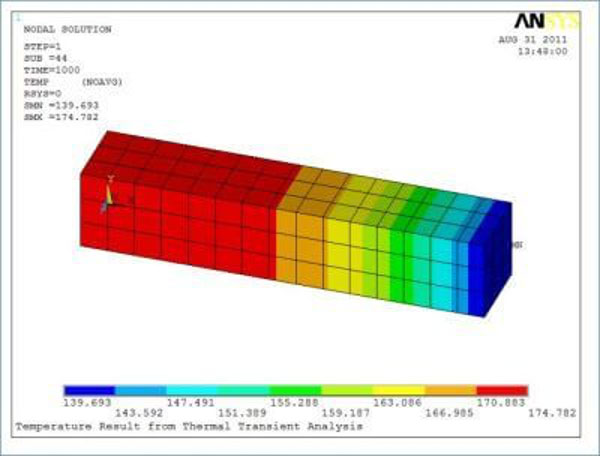
Such plots can be followed by animations of results. Results from the RTH thermal results file will often be wanted for use in stress analysis, in order to determine the range of thermal stresses that result in a model.
Summary
This document has described the independent planning of times at which convective heat transfer coefficient and bulk temperature will change, for use in a transient thermal finite element analysis. Step changes can be described with a value change in a relatively short time interval. Gradual changes will be managed by the ramping provided by Table Arrays that use Time variation of values. Substeps employed by the Ansys transient solver will follow the Table Array load curves.
Solutions will be formed at important times in the Table Arrays if the TSRES command uses an array of the times in all Table Arrays that describe time-dependent loading. The procedure lets a user represent complex plans for equipment operation in transient thermal analysis.
Appendix
Users may prefer to truncate the amount of data written to the RTH file by OUTRES. The following code illustrates setting a user-entered max_delta value that indicates the longest time interval before another data point is written to the RTH file.
The existing myTSRES array is checked to see whether the max_delta value exceeds the length of any time interval, and if so, extra solution points are inserted. The resulting array newTS is used for both the TSRES and OUTRES commands. The user must ensure that max_delta is greater than the minimum time interval in the DELTIM command.
! Form a numerical Array for times for TSRES commands
! Solutions will be formed at these times, plus others as further below
! Use ALL the times in both the “my_conv” and “my_bulk” Table Arrays
! The ZERO time is not required
!
*dim,myTSRES,array,7 ! Dimension a numerical Array, 7 rows, 1 column
!
myTSRES(1)= 120 ! as found in both arrays
myTSRES(2)= 130 ! as found in my_conv array
myTSRES(3)= 500 ! as found in my_bulk array
myTSRES(4)= 700 ! as found in both arrays
myTSRES(5)= 710 ! as found in my_conv array
myTSRES(6)= 900 ! as found in my_bulk array
myTSRES(7)=1000 ! as found in both arrays
*get,numrows,PARM,myTSRES,DIM,X ! how many rows in “myTSRES”
lasttime=myTSRES(numrows) ! what is the last time in “myTSRES”
max_delta=50 ! preferred Delta_T for OUTRES, larger then minimum in DELTIM
*dim,my_out,array,numrows+NINT(lasttime/max_delta)+1 ! large enough plus extra space
prev=0
jj=0
*do,ii,1,numrows
interval=myTSRES(ii)-prev
*if,interval,LE,max_delta,then
jj=jj+1
my_out(jj)=myTSRES(ii)
prev=myTSRES(ii)
*else
numsteps=NINT(interval/max_delta+.49999999999999)
int=interval/numsteps
*do,kk,1,numsteps-1
jj=jj+1
my_out(jj)=prev+kk*int
*enddo
jj=jj+1
my_out(jj)=myTSRES(ii)
prev=myTSRES(ii)
*endif
*enddo
! Find row number of last non-zero entry in “my_out”
*VSCFUN,myLAST,LAST,my_out(1)
*dim,newTS,array,myLAST
*VFUN,newTS(1),COPY,my_out(1) ! gets rid of zeros on the end
TSRES,%newTS% ! force transient solve to include these times
! Use percent signs “%” arround Array name
OUTRES,ERASE
OUTRES,ALL,NONE
OUTRES,ALL,%newTS% ! write all the values as in TSRES
Further enhancement would be APDL programmed construction of the myTSRES array from the contents of the table arrays for the convective heat transfer coefficients and the bulk temperatures.
Additional Ansys Software Tips & Tricks Resources
-
- Analyzing normal and Tangential Elastic Foundations in Mechanical
- Importance of Meshing for Structural FEA and Fluid CFD Simulations
- For support on Contained Fluid FEA Modeling with HSFLD242 Elements
- For Exporting a Deformed Geometry Shape Post-Analysis in Mechanical
- For guidance Multi-Step Analyses in Mechanical
- For Retrieving Beam Reaction Force in a Random Vibration Analysis
- How to display the Vortex Core Region in Ansys Mechanical
- Deploying Ansys Macro Programming vis *USE Command in Mechanical
- For replicating Fatigue Models from Start to Finish in Mechanical
- Setting up Acoustic Simulations of a Silencer
- For a step-by-step guide on 2D to 3D Submodeling in Mechanical
- For modeling Pipe16 Circumferential Stress in Mechanical
- For Support on performing ‘EKILL‘ in Workbench
- APDL Command Objects post-Spectral Analysis
- For Separating DB Database Files from RST Files
- Measuring Geometric Rotation in Mechanical WB
- Explicitly, CAD Geometry Deformation Plasticity
- Offsetting a Temperature Result to Degrees Absolute
- For general guidance on Ansys Post-Processing
- Finally, for basic Ansys Software Installation and License Manager Updates